

The Object Properties palette displays the properties of the currently selected object. Which fields are visible depends on the selected object type. If multiple objects are selected at the same time, the palette shows the shared or combined properties of this selection.
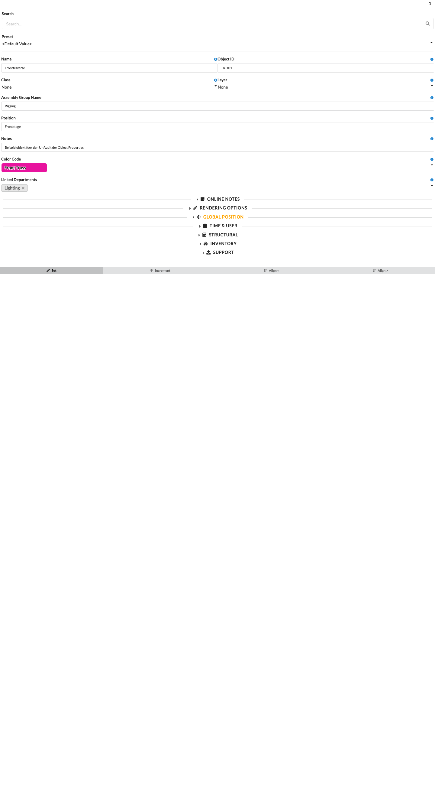
| Panel/Field | Detailed Description |
|---|---|
| Panel Groups | Show the properties in the order used by the interface. Which groups appear depends on the selected object type, its geometries, and the available connections. |
| Search and Input Panel | In the upper part of the palette, you can directly edit the most important properties of the currently selected object. Depending on the object, this includes name, ID, assignments, and technical parameters. |
| Value Panel | In the middle and lower part, the actual setting fields appear. There you can change properties, review them, or link them to other objects. |
| Object-Dependent Content | The screenshot shows an example view. In your project, more or fewer fields may be visible because Production Assist only shows the properties that are relevant to the selected object type. |
You can use almost all text drop-down menus in the Object Properties as a search field. Click in the field and type a term. Only matching entries will then be displayed. If no entry matches your term, an Add appears in front of it. Press Enter to create this term as a new entry. Typical examples include the drop-down menus for layers or classes.
You can expand and collapse each area of the palette using its heading. In table views, a small arrow also appears in the group heading so you can quickly open or close related blocks.
The general information is displayed for all object types. The number in the upper filter area indicates how many objects are currently selected. In a narrow mobile layout, the number, Search, and Preset appear on one line; the search field uses most of the available width.
The current example image shows the fields that are always visible: Search, Preset, Name, Object ID, Class, Layer, Assembly Group Name, Position, Notes, Color Code, and Department. Each field is explained in the panel below. The internal UUID in the version history is separate from the editable Object ID.
The search field allows you to filter the palette for specific properties.
The field shows which preset value currently applies to the object. By default, it shows Default. This means no special preset is being used.
To learn how to create and activate object presets, see Presets in Navigation.
These fields show the Name and the Object ID of the selected object. Both values can also be changed here. The Object ID is always displayed before the Name in the Scene Tree. If it appears in red, it has been assigned more than once in the plan.
These fields show which layer and class the object is on. Both values can be changed here. You control visibility in Navigation under Classes and Layers.
Shows the name of the assembly group in which the object is located.
Here you can assign a Color Code to objects or assembly groups for the Paperwork. This is primarily used in touring productions.
Each object can be assigned a Department for later Paperwork.
| Panel/Field | Detailed Description |
|---|---|
| Search | Filters the displayed properties within the palette. This is particularly helpful when many fields are visible and you want to quickly jump to a specific property. |
| Preset | Shows which preset value currently applies to the object. By default, it shows Default; this means no special preset is being used. |
| Name | Sets the visible name of the object. This name appears later in lists, in the Scene Tree, and in the Paperwork. |
| Object ID | Shows or changes the unique identifier of the object. It is primarily used for unique assignment and stands out immediately in the Scene Tree if it has been assigned more than once. |
| Class | Assigns the object to a class. This is mainly used to control visibility, structure, and filters in the drawing. |
| Layer | Assigns the object to a layer. This is important for organizing objects cleanly in larger projects. |
| Assembly Group Name | Shows or changes the name of the assembly group to which the object belongs. This helps with logically grouping related objects. |
| Position | Stores a free position designation for lists, labels, and Paperwork. Here you can enter, for example, a descriptive mounting or deployment position. |
| Notes | Stores internal notes directly on the object. This information helps with handovers, special cases, or team inquiries. |
| Color Code | Color-marks objects for planning and Paperwork. This allows you to quickly identify, for example, tour segments, responsibilities, or object groups. |
| Linked Departments | Assigns the object to one or more departments. This makes it clear which team or work area is relevant for the object. |
| Hang at Center | Aligns a symbol or fixture with the center of the truss. This field appears only for suitable symbol or fixture types. |
Additional properties appear for label objects and when editing a label template. For the full procedure for creating and printing labels, see the label guide.
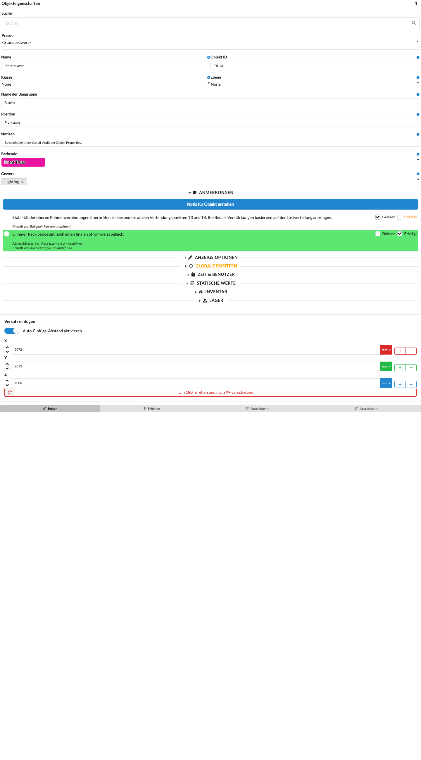
You can store notes about objects here.
| Panel/Field | Detailed Description |
|---|---|
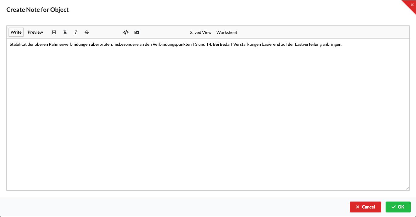
| Create Note for Object | Opens the Markdown editor for a local note on the selected object. Write the text in the Write tab and, if needed, check the formatting under Preview. OK creates the note on the object. This is suitable for internal information that should be kept with the project. |
| Object-Related Information | The screenshot shows that notes can be maintained directly in the object information. This keeps notes right where they are needed. |
| Read / Done | Show or change the processing status of existing notes. The current example screenshot contains synthetic entries with different statuses. |
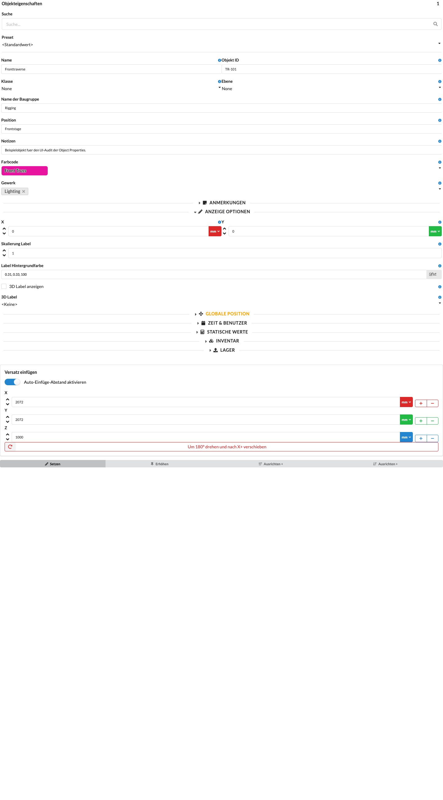
Under Rendering Options, you control the position and appearance of labels directly on the object.
| Panel/Field | Detailed Description |
|---|---|
| X | Sets the horizontal label offset. This lets you position the label neatly beside the object. |
| Y | Sets the vertical label offset. This lets you fine-tune the label position in the plan. |
| Label Scale | Scales the size of the label. This is useful when labels need to appear larger or smaller depending on the scale. |
| Label Background Color | Sets the background color of the object label. |
| Show 3D Label | Shows or hides the assigned 3D label in the model. |
| 3D Label | Selects the label template assigned to the object as a 3D label. |
The Transform panel contains all information about the object's position, scale, and rotation. The units are color-coded according to their respective axis.
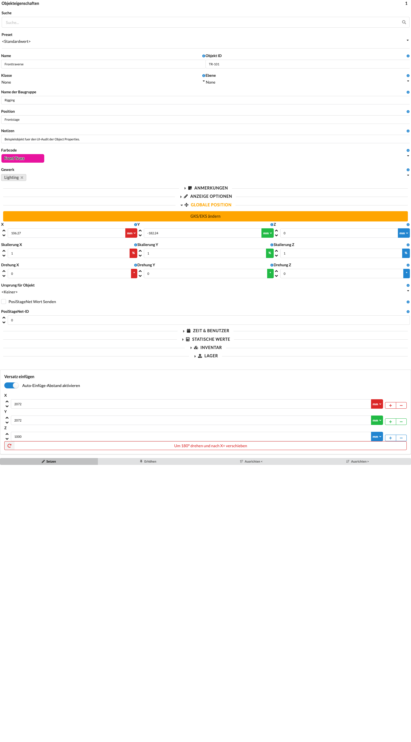
Use Change GCS/LCS directly in the Position or Global Position section to change the coordinate reference used by the fields. The Global Transformation setting under Settings controls the same mode.
With global transformation, the values refer to the drawing coordinate system. With local transformation, they refer to the object or its parent object. This is especially important when an object is part of a rotated or moved structure; the global Z value is not automatically its height above a ground surface.
| Panel/Field | Detailed Description |
|---|---|
| X, Y, Z | Set the object's exact position along the three axes, allowing you to move it precisely in space. |
| Scale X, Scale Y, Scale Z | Scale the object along the X, Y, and Z axes. These fields are useful when an object needs to be adjusted or mirrored. |
| Rotation X, Rotation Y, Rotation Z | Rotate the object around the respective axis so you can align it precisely as needed. |
| Origin Reference | Defines the reference point from which the position offset is calculated. This lets you measure and position objects correctly using defined reference points. |
| PosiStageNet Send Value | Enables the output of position data via PosiStageNet. This option is only relevant when Production Assist is working as a sender. |
| PosiStageNet ID | Shows the object's PSN ID. When Production Assist is used as a client, this value can be used or set; when Production Assist sends, the ID is assigned automatically. |
Enable PosiStageNet Send Value on objects whose position data should be sent. Leave this option disabled on the receiving side; there, PosiStageNet ID assigns the target object to the incoming tracker. The sending and receiving objects use the same ID.
For complete instructions for the sender and receiver, footer controls, history views, and troubleshooting, see Send and Receive PosiStageNet.
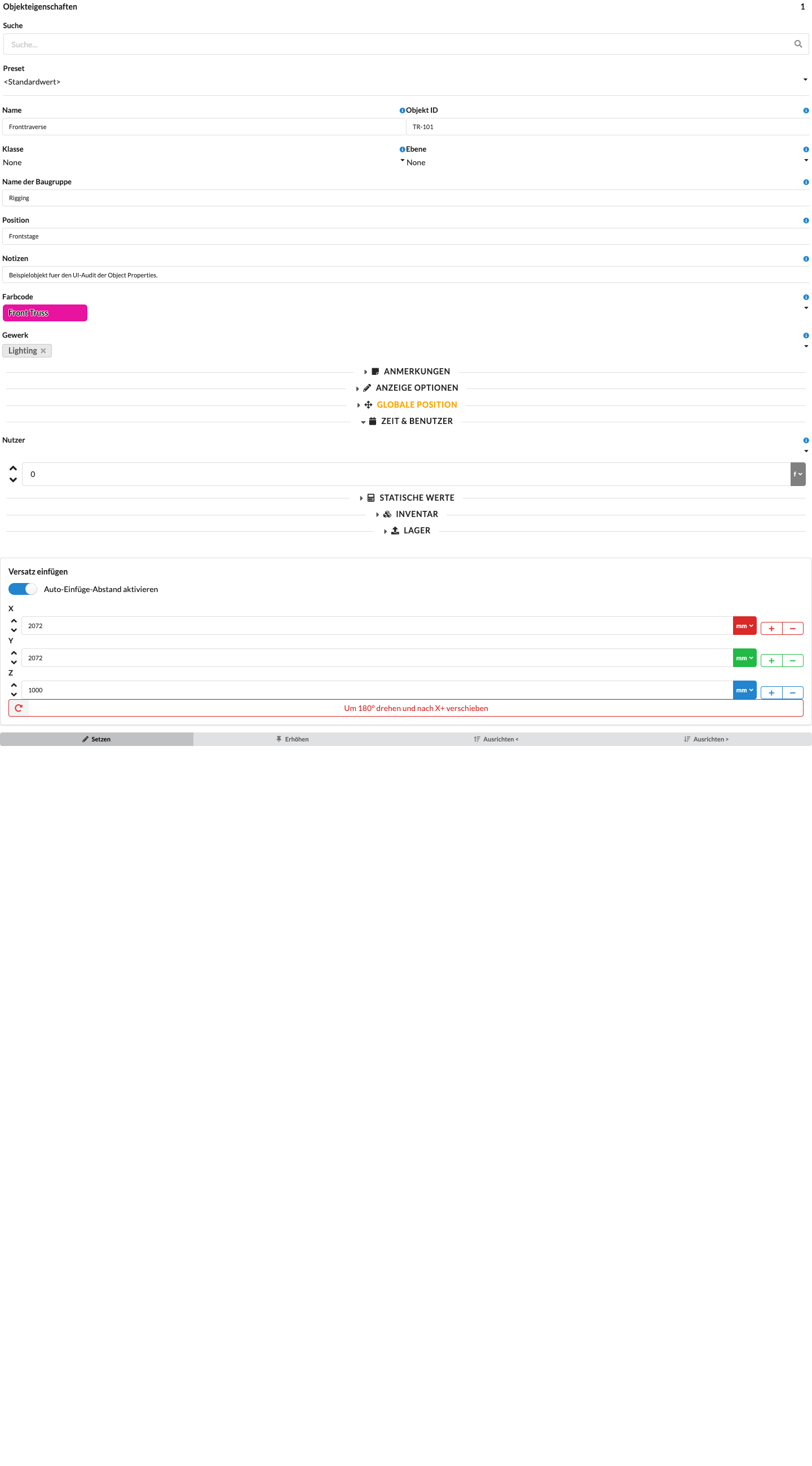
You can assign a person under User and an estimated work duration under Duration to each object or Assembly Group. You can use this information in Worksheets to assign work packages and evaluate the expected time required.
First, add the person as a drawing user in the Users tab of Navigation. No online project is required. If the responsibility should also be used in online tasks, link the drawing user to a Production Assist account and an online project as well. Project access and user assignment are separate settings.
| Panel/Field | Detailed Description |
|---|---|
| User | Assigns a person responsible for the object, making it clear who is handling the object or work package. |
| Duration | Stores the planned work time for setup, handling, or processing. This information is useful for estimates, scheduling, and later evaluations. |
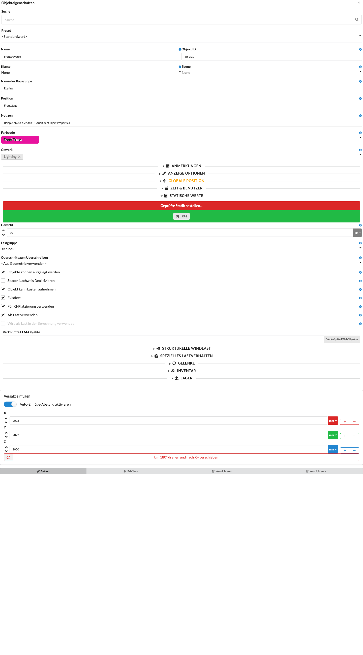
For objects relevant to structural calculations, this section contains fields for weight, load group, structural behavior, and wind load. The options shown depend on the geometry and object type.
| Panel/Field | Detailed Description |
|---|---|
| Request Reviewed Structural Calculation | Use this function to request a reviewed structural calculation. This is relevant when a formal proof of structural stability is required in addition to the internal calculation. In that case, Production Assist's internal engineering office performs the review. For more information, see Static Office. |
| Weight | Sets the object's weight. This weight is included directly in the load calculation. For Bridles, when accepting the parts preview and during automatic parts assignment, the total weight of all components, including the Basket, shackles, and Drop, is entered. Incomplete subtotals do not overwrite the existing value. |
| Load Group | Assigns the object to a load group. The load-group factor is multiplied by the load factor and by the group factor and, where applicable, the layer factor of the active load combination. A load-group factor of 0 in the load combination excludes that group from the combination. |
| Override Cross Section | Manually overrides the cross section used for the calculation. This is useful for quickly checking different variants without changing the object's symbol or geometry. However, this function is only of limited use for objects with several different structural members, because it overrides all cross sections of the object together. |
| Objects Can Be Placed On Top | Determines whether other structural members can be placed on this object. When enabled, the object can serve as a receiving or supporting member in the model logic, allowing Production Assist to create Truss Cross connections between it and other suitable objects. |
| Disable Spacer Verification | Disables structural verification calculations for truss spacers on this object. Normally, all short trusses and spacers are included, which reduces the calculated load-bearing capacity. If the truss segment has bracing, enable this option so that its full load-bearing capacity can be calculated. |
| Object Can Receive Loads | Determines whether loads can be attached to this object and included in the calculation. This is useful for controlling automatic load assignment and excluding specific objects from receiving loads. |
| Group Loads in Structural Assembly | Groups the loads within the structural assembly to organize the calculation. |
| Exists | Hides the object from the renderer and Scene Tree and excludes it from the structural calculation. The object remains saved in the drawing and can be shown and included again by re-enabling this option. |
| Use for AI Placement | Determines whether this structural object is a possible location for Rigging → Place Hoists on Structure. Disable the option to exclude the object from this automatic support placement. Pipes are also controlled by the global setting Use Pipes for AI Hoist Placement. |
| Use as Load | Determines whether the object's weight is included as a load in the calculation. When disabled, the object remains in the model for other purposes, but its weight is not included. |
| Used as Load in Calculation | Indicates whether the object is currently included as a load in the calculation. This is a read-only field that is set automatically and is for information only. |
| Linked FEM Objects | Shows linked FEM objects, so you can see which other calculation elements are related to this object. |
| Truss Cross Type | Determines whether placed truss connections are flexible, compression-only, tension-only, rigid, or excluded from the calculation. This field appears when a Truss Cross is present. |
| Transferred Force – Design Value | Shows the factored force transferred through the Truss Cross. |
| Transferred Force – Characteristic Value | Shows the characteristic, unfactored force of the Truss Cross. |
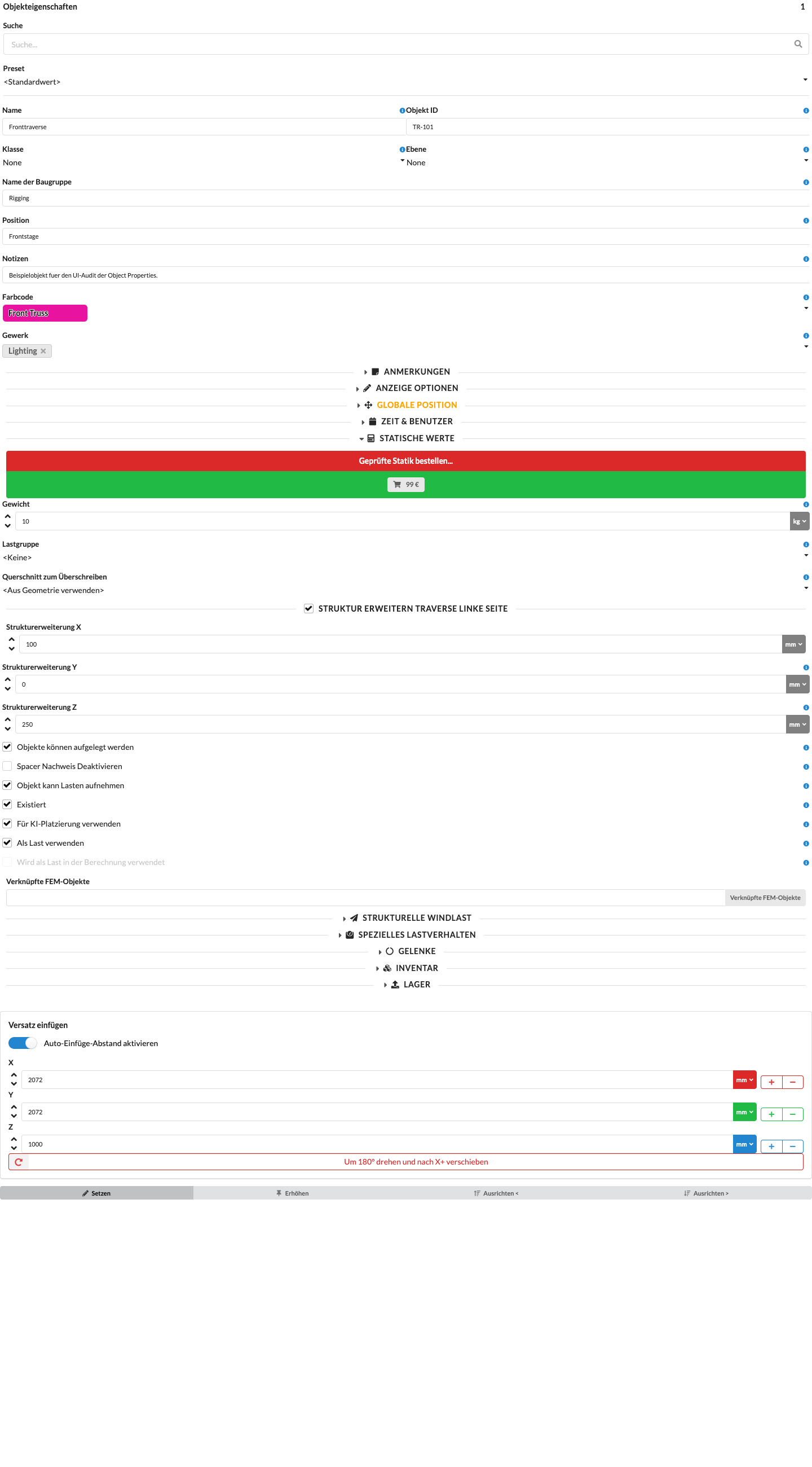
For magnetically connected structural members, an extension option and its X, Y, and Z offsets are also shown. The offsets adjust the structural geometry for the calculation and use the magnet's coordinate system.
| Panel/Field | Detailed Description |
|---|---|
| Extend Structure – [Name] | Enables an extension for the specified magnetically connected structural member. |
| Extension Offset X, Y, Z | Sets the extension along the three axes of the magnet's coordinate system. The offsets are shown only when the extension option is enabled. |
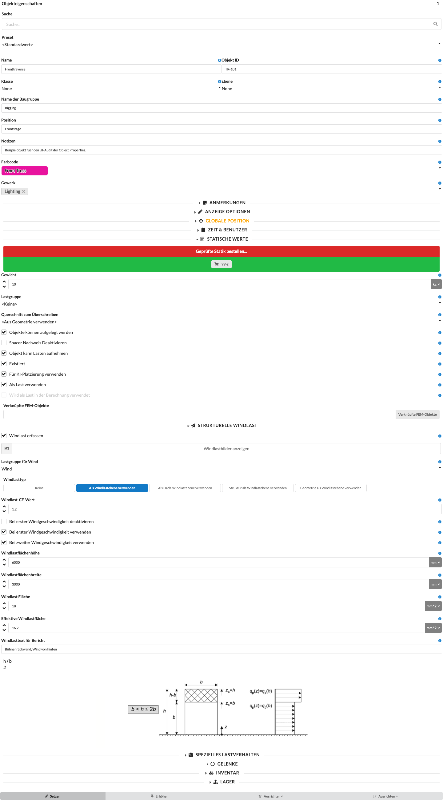
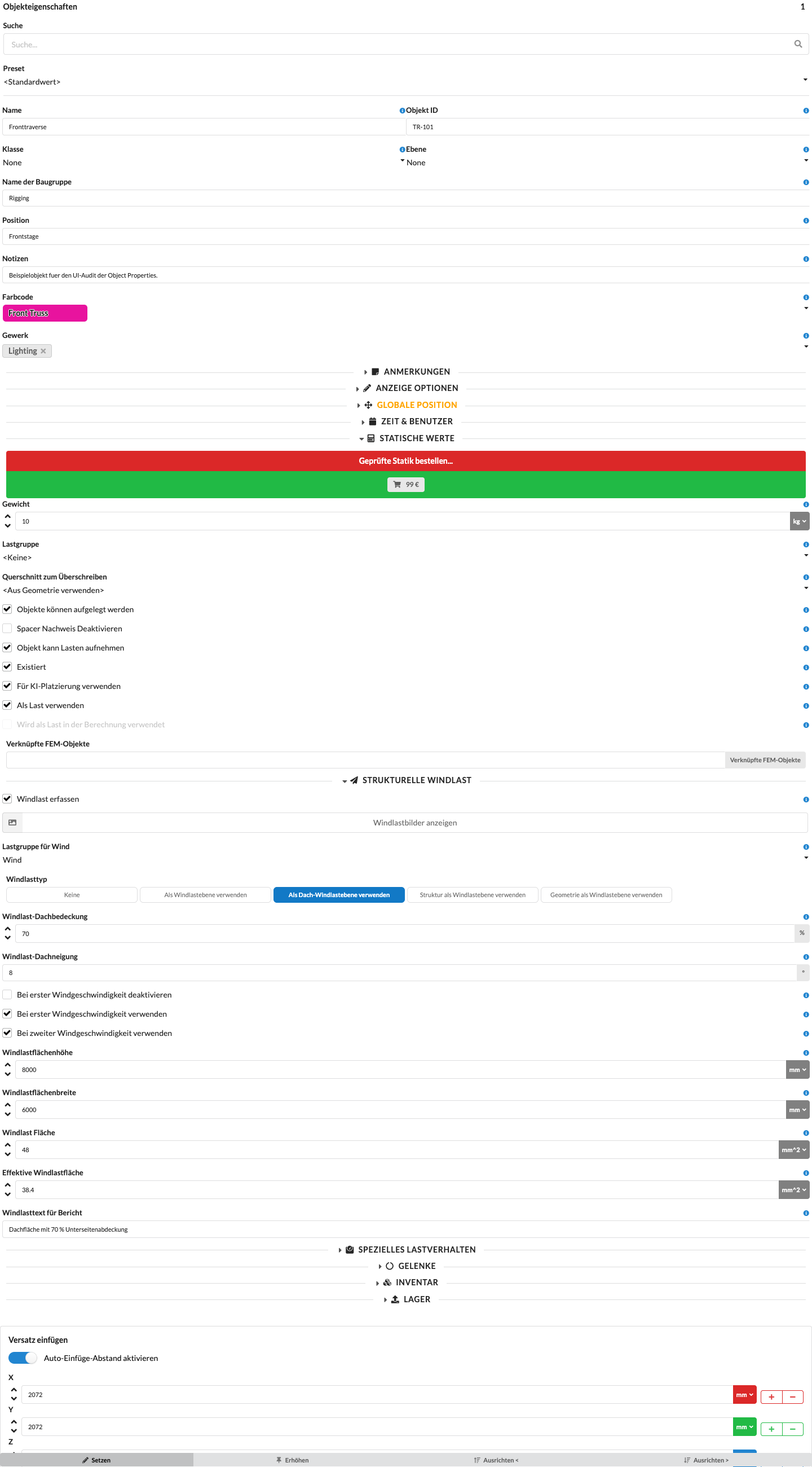
| Panel/Field | Detailed Description |
|---|---|
| Apply Wind Load | Controls whether the structural members of this object receive wind load. Disable the option for individual members that should not receive wind load, such as scaffold diagonals. Set the wind plane and its geometry separately using the following selection fields. |
| Show Wind Load Images | Opens the wind load case views so you can check the areas and directions used. |
| Wind Load Group | Determines which load group receives the wind loads generated by this object, so the appropriate safety and combination factors are applied to the wind loads. |
| Wind Load Type | Selects from None, Use as Wind Plane, Use as Roof Wind Plane, Use Structure as Wind Plane, and Use Geometry as Wind Plane. The selection determines which additional area fields appear. |
| Use as Wind Plane | Defines the object as a wind load area to which wind pressure is applied. This option is particularly suitable for banners, walls, or other closed surfaces with 2D polygon geometry. |
| Use as Roof Wind Plane | Uses a 2D polygon as a roof area for roof wind loads. Wind pressure is applied uniformly over the horizontal reference area. Depending on the load-combination settings, the load acts perpendicular to the roof surface as suction away from the roof or pressure toward it. |
| Use Structure as Wind Plane | Determines the wind area from the underlying structural geometry. This is particularly useful for trusses, frameworks, and other load-bearing equipment because it takes width, height, and, where applicable, bracing into account. |
| Use Geometry as Wind Plane | Uses the object's 3D geometry as the basis for wind load calculation. Depending on the wind direction, the 3D body is projected onto a wind plane, allowing the effective area to be determined based on the direction of the wind. |
| Wind Load Roof Coverage | Only for a roof wind plane: describes the coverage under the roof, from 0% (freely ventilated) to 100% (closed or blocked underneath). It affects the calculated roof coefficient in the suction case. |
| Wind Load Roof Pitch | Only for a roof wind plane: shows the pitch calculated from the roof geometry for the wind direction. This value cannot be entered manually. |
| Wind Load CF Value | Sets the aerodynamic force coefficient for wind planes outside roof mode. For a roof wind plane, Production Assist calculates the roof coefficient from the roof pitch and load direction; the underside coverage affects the suction case. |
| Disable at First Wind Speed | Suppresses wind loads generated by this object in the first wind load case. The object itself remains within the calculation scope. |
| Use at First Wind Speed | Determines whether the object is included in the calculation scope of the first wind load case. If you disable the option, the object is not considered in that wind load case. |
| Use at Second Wind Speed | Determines whether this object's wind load is considered in the load case for the second wind speed. This is useful for simulating changed conditions at higher wind speeds, such as banners being removed later. |
| Wind Load Area Height | Shows the height of the effective wind load area. This value is calculated automatically and is for checking purposes. |
| Wind Load Area Width | Shows the width of the wind load reference area. Together with the height, this lets you understand the geometric basis used to determine the wind pressure distribution in the verification. |
| Wind Load Area | Shows the total area used for this object's wind load calculation. This automatically calculated value is mainly for checking the effective area exposed to the wind. |
| Effective Wind Load Area | Shows the effective wind load area used after internal reductions or derivations. |
| Wind Load Text for Report | Stores text for the structural report, allowing object-specific notes to be included directly in the report. |
Check the geometry and applied areas under Wind Loads and Wind Load Areas. Set the wind cases and factors active in the calculation under Load Combinations.
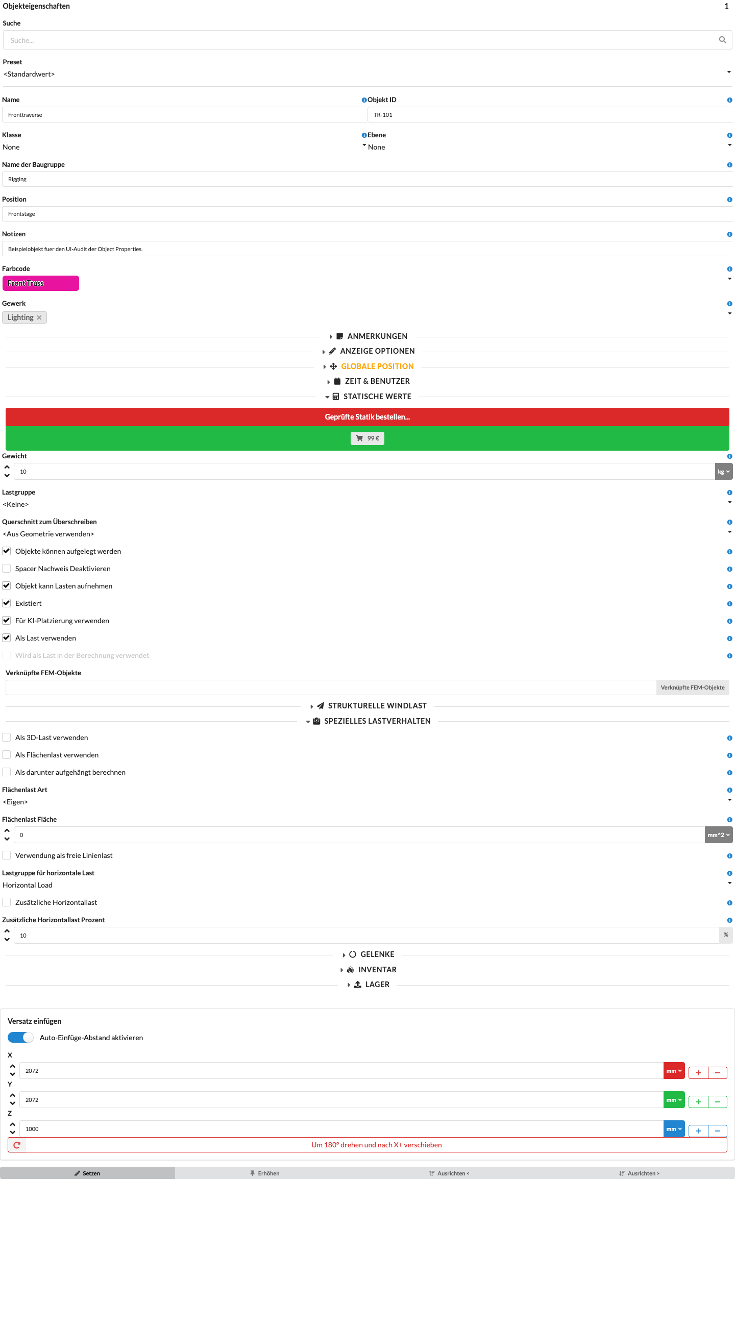
| Panel/Field | Detailed Description |
|---|---|
| Use as 3D Load | Uses the object's 3D body to distribute its weight as a spatial load in the calculation. Enable this option when the 3D geometry represents the actual load distribution better than a single attached load. |
| Use as Area Load | Uses a polygon of the object as an area over which its weight is distributed. The object must contain at least one polygon geometry. Structural members adjoining the polygon area receive portions of the load. |
| Calculate as Suspended Below | For area and 3D loads, accounts for the object being suspended below the supporting structure. For example, use it for a banner under a truss if the greater vertical distance would otherwise prevent the load from being assigned to the structure. |
| Area Load Type | Selects an additional, flat-rate area load: Custom, the listed values under EN 13814, or load classes 1 to 6 under EN 12811. Custom applies no additional flat-rate value. The standard values supplement the object's weight; they do not replace it. |
| Area Load Area | Shows the area calculated from the polygon geometry. Production Assist calculates this value; it cannot be edited directly. |
| Use as Free Line Load | Uses the object's line as a free-standing line load. The line must touch or intersect structural members so Production Assist can connect the load to the structure. If the load cannot be connected, the calculation stops with an error. |
| Horizontal Load Group | Assigns additional horizontal loads and horizontal equivalent loads generated by load combinations to a load group. The group factor is multiplied by the relevant load-combination factors. |
| Additional Horizontal Load | Enables an additional horizontal load component for the object. This component is derived from the object's vertical loads and scaled by Additional Horizontal Load Percentage. |
| Additional Horizontal Load Percentage | Sets the percentage of the object's vertical load to be applied as an additional horizontal load. |
For a detailed explanation with examples, see Area Load, 3D Load, and Suspended Load. It also explains how the geometry must connect to the structure. For load group and load combination settings, see Load Combinations.
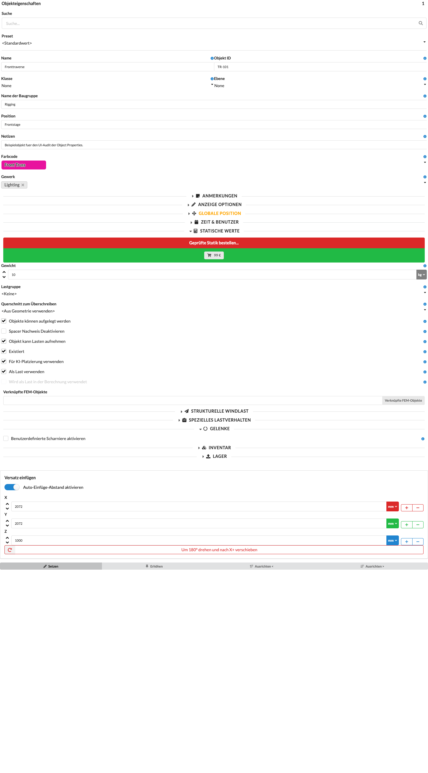
| Panel/Field | Detailed Description |
|---|---|
| Enable Custom Hinges | Displays individual hinge options for each structural member of the object. Enable the option only when you need to adjust force transfer at the connections. |
| Hinge Nx, Vy, Vz, Mt, Mby, Mbz | Releases the respective force or moment component at the connection. The options appear for each structural member when custom hinges are enabled. |
When you enable Enable Custom Hinges, the six options Hinge Nx, Hinge Vy, Hinge Vz, Hinge Mt, Hinge Mby, and Hinge Mbz appear for each structural member. Enable the components that should be released as hinges at each connection. These values are used when building the structural model. Leave the default settings unchanged if you do not have a professionally reviewed specification for the connection.
Open Object Properties → Hinges, enable Enable Custom Hinges, and select Connection Springs… for the relevant structural member. The same dialog is available next to the hinge options when editing a structural geometry.
The dialog edits the components Nx, Vy, Vz, Mt, Mby, and Mbz in the member's local axes. The spring connects the end of the member to its calculation node. Its deformation is the relative translation or rotation between these two points.
| Dialog selection | Behavior |
|---|---|
| Use Existing Hinge Setting | Inherits the setting from the structural geometry at the object level, and there the connection specification from the cross-section template. If no explicit mode is set, the existing hinge checkboxes apply. The stored Layher K2000+ profiles therefore use their connection springs automatically. |
| Rigid | Connects the component rigidly. An existing hinge checkbox is overridden for this component. |
| Released | Releases the component completely. |
| Linear Spring | Uses constant stiffness. Enter N/mm for translations and N·mm/rad for rotations. A stiffness of zero is equivalent to a release. |
| Piecewise Linear Spring | Connects the entered value pairs with straight lines. For translations, the table uses mm and N; for rotations, it uses rad and N·mm. |
In the Connection Springs… dialog, Spring Template provides predefined springs for Layher K2000+. They are based on the characteristic curves in Appendix A, Figures 3 to 8, of the DIBt document Z-8.22-64 dated April 23, 2018. Selecting a template creates an editable copy for exactly one component. The other components retain their values. No complete connection or assembly is created.
The cross sections Layher - O Riegel K2000+, Layher - O Riegel K2000+ Enforced, Layher - U Riegel K2000+, and Layher - U Riegel K2000+ Enforced automatically apply these specifications at both ends. Both beam types use the springs for Vy, Mby, and Mbz; O-beams also use the clearance curve for Mt. For U-beams, Mt is released. For beams shorter than 600 mm, all three rotational components are released; the shear spring remains. At 600 mm and above, the rotational springs apply. Explicit settings on the geometry or object can override these specifications.
The cross section Layher - Dubbele Spiekop includes the cDK rotational spring for Mby at both ends. The Vz slip approximation, Vy, and Mbz are each specified only at the start, so their flexibility is not counted twice; Mt is released at both ends. You still need to model the specified substitute-model distances and rigid intermediate pieces. The Vz specification is the same explicitly designated numerical approximation shown in the template table. Other Layher profiles, such as standards, diagonals, or welded transoms, do not receive these springs automatically. The specifications are visible under Resource Manager → Cross-Section Templates in Details. Previously saved explicit connection modes retain precedence; after loading, inherited connections on the named standard profiles use the new specifications.
| Template / component | Stored characteristic curve and mapping |
|---|---|
| Beam/bracket connection, Mby, Figure 3 | Piecewise linear approximation of φ = My / (9140 − 73.6 · \ |
| Horizontal bending, Mbz, Figure 4 | Linear rotational spring with 5,100,000 N·mm/rad for the beam/bracket connection and double-wedge-head coupler. |
| O-beam/U-bracket connection, Mt, Figure 5 | Moment-free range between −0.0629 and +0.0629 rad, followed by 10,910,000 N·mm/rad. The positive source curve is mirrored for negative moments. This template does not apply to U-beams or double-wedge-head couplers. |
| Horizontal shear, Vy, Figure 6 | Linear translational spring with 4,850 N/mm for the beam/bracket connection and double-wedge-head coupler. Stiffness does not replace a resistance check; among other values, the source distinguishes 10 kN for O-beams/U-brackets and 5.9 kN for U-beams. |
| Double-wedge-head coupler, Mby, Figure 7 | One cDK rotational spring in the substitute model; piecewise linear approximation of φ = My / (2500 − 19 · \ |
| Double-wedge-head coupler, Vz, Figure 8 | Approximation of the slip model explicitly described as a numerical slip approximation, with ±5,100 N friction resistance and ±3.6 mm slip travel. The ideally rigid sections are approximated with 1,000,000 N/mm; force increases by 5.1 N (0.1%) over the slip segment. These stiffnesses are numerical assumptions, not manufacturer specifications. |
The two curved bending curves are mirrored about the origin. Within the tabulated ranges, their relative moment error due to linear interpolation is at most 0.2%. Outside the tables, the extended end segments of the general spring model apply. The displayed reference ranges do not limit forces or trigger an automatic resistance or interaction check.
According to the source drawing, the spring for the beam/bracket connection is 25 mm from the standard axis. The substitute model for the double-wedge-head coupler requires two cDK rotational springs: 43 mm from each standard axis to its respective spring and 68 mm between the springs, for a total of 154 mm. Model this geometry with rigid intermediate pieces and exactly one slip component; neither the template selection nor the cross-section specifications create this geometry. If slip is modeled separately at the center, remove the inherited Vz spring at the start by explicitly setting the mode to Rigid, so it does not act twice. The drawing for the vertical diagonal also specifies ex = 77 mm and ey = 50 mm for K2000+. Figures 3 to 8 and the system diagram do not provide a numerical diagonal spring; no spring stiffness is invented for it.
The Vz approximation is continuous and reversible. It models neither the exactly discontinuous inverse relationship in Figure 8 nor a friction history. The source allows vertical shear forces above the friction resistance of 5.1 kN only under non-reversing loading. Therefore, do not use the template to verify reversing or cyclic slip loading.
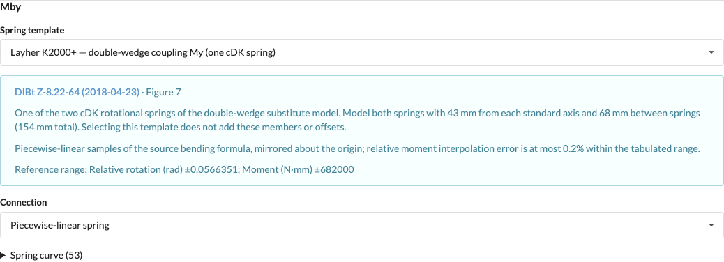
The following images show the English-language interface; the names used in the procedure correspond to the English interface.
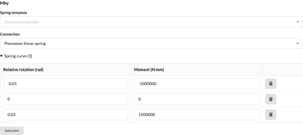
The image shows example values for Mby; they are not a specification for a particular connection.
To define a force-dependent spring:
The spring uses the same curve during loading and unloading. It does not model permanent deformation or hysteresis. The stability check uses the actual curve slope, including on horizontal curve segments. A helper stiffness for the equilibrium iteration does not count as additional connection stiffness. At curve kinks, the softer adjacent slope is applied conservatively; calculation may therefore stop there. The check applies to the modeled subdivision of members into calculation elements; adding more display points to a result curve does not improve the kink calculation. Outside the entered points, the first or last straight line continues with unchanged slope. Descending curve segments and non-finite numbers are not allowed; Apply remains disabled for invalid entries.
Explicit modes on the object override the connection setting of the structural geometry, which in turn overrides the cross-section connection specifications. Use Existing Hinge Setting restores inheritance from the preceding level. An explicit mode takes precedence over a hinge checkbox. The six existing checkboxes remain available as a fallback when no level specifies an explicit mode.
Nonlinear spring calculation also works when second-order calculation is disabled. If the ∆P method is enabled, both effects are considered together. Calculation may stop if equilibrium cannot be reached or the system is unstable; in that case, check the curve, supports, and loads. Section forces show the forces and deformations of the member, including its spring connections.
Structural export to DSTV or IFC does not currently support these spring models and stops when a model contains connection springs. The settings are retained when saving the Production Assist drawing.
In the Paste Offset area, set the offset for the duplicate commands on the X, Y, and Z axes. Enter the desired distance on each axis, then use the plus or minus button to duplicate the selected objects in that direction. Flip 180deg and Move X+ duplicates the selection, rotates the copies by 180°, and moves them in the positive X direction. The commands are also available from Edit → Duplicate. Keyboard shortcuts depend on the active CAD integration and the shortcuts configured there.
With the native copy and move commands in AutoCAD and BricsCAD, the command first asks you to select blocks if nothing is preselected. Then press Enter to use the existing Paste Offset or enter a new distance directly in the CAD command line. A new entry updates the selected axis's Paste Offset in Production Assist. Enter the distance in drawing units; Production Assist converts it to millimetres. The native commands follow the axes of the current user coordinate system (UCS). The positive command increases the chosen UCS coordinate by the positive distance; the negative command decreases it. The command stays active after each action: press Enter once to repeat using the last confirmed distance. Esc finishes the command; completed actions and confirmed distances remain.
Enable Auto Paste Offset automatically adjusts the paste offsets to the X, Y, and Z extents of the selected structural geometry. This is useful when you want to arrange copies directly next to each other. The manually entered axis offsets remain available when automatic adjustment is turned off. The same option is available under File → Settings... → Renderer.
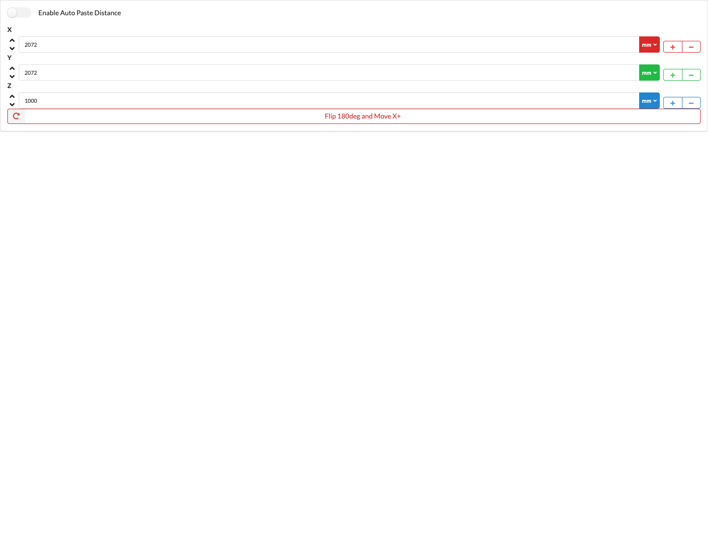
| Panel/Field | Detailed Description |
|---|---|
| Paste Offset X | Sets the distance for duplicates in the X direction. The X+ and X− buttons duplicate the selection using this distance. |
| Paste Offset Y | Sets the distance for duplicates in the Y direction. The Y+ and Y− buttons duplicate the selection using this distance. |
| Paste Offset Z | Sets the distance for duplicates in the Z direction. The Z+ and Z− buttons duplicate the selection using this distance. |
| Enable Auto Paste Offset | Automatically adjusts the paste offsets to the X, Y, and Z extents of the selected structural geometry. The option is also available under File → Settings... → Renderer. |
| Flip 180deg and Move X+ | Duplicates the selection, rotates the copies by 180°, and moves them by the positive X paste offset. |
The Inventory panel contains all parameters relevant to logistics.
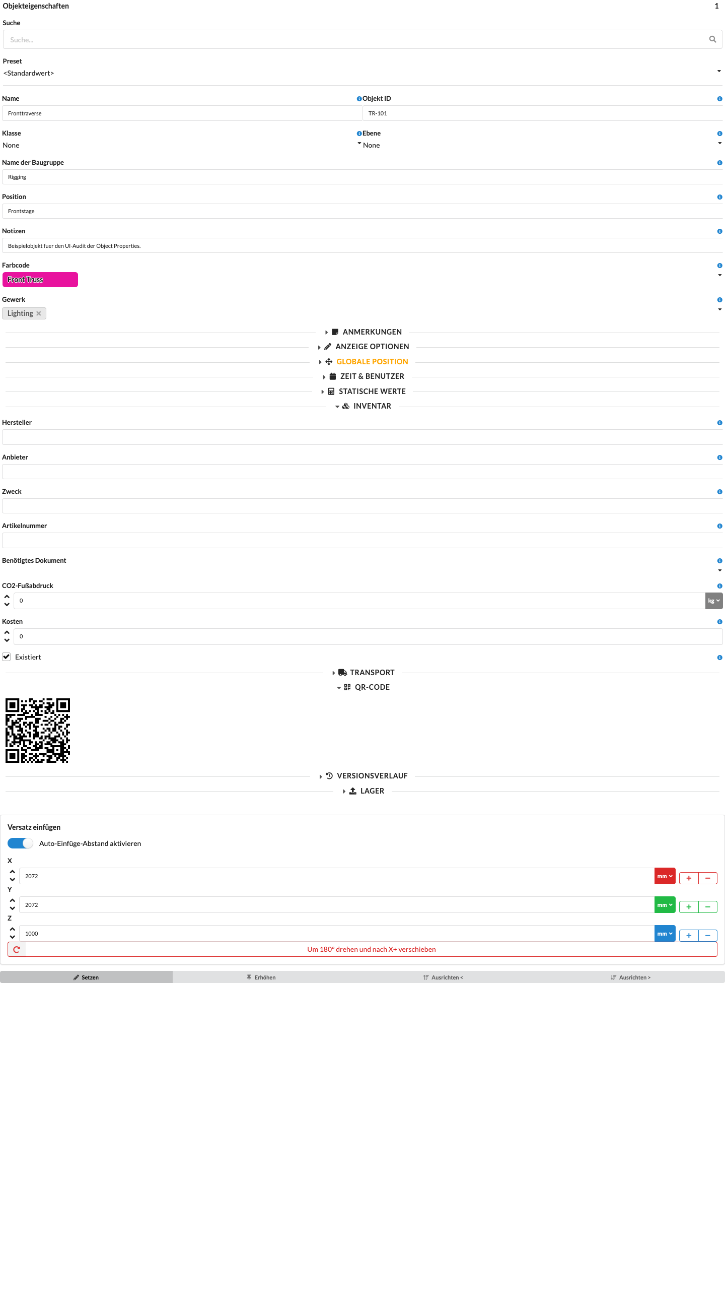
| Panel/Field | Detailed Description |
|---|---|
| Manufacturer | Stores the object's manufacturer. This field helps you later evaluate material by brand or origin. |
| Supplier | Stores the object's supplier so you can track where the material was sourced. |
| Purpose | Describes the object's intended use. This is useful when an object needs to be categorized by function as well as name. |
| Part Number | Stores the article or part number, making it easier to compare objects with warehouse or ERP data. |
| Use as Cable Definition | Marks the object as a cable definition that can be used for cable planning. |
| Accepted Excess Cable Length | Sets how much excess length is accepted when a cable is assembled automatically before shorter cable segments are added. |
| Needed Document | Links inspection reports, certificates, or other documents to the object so important records remain accessible from the relevant entry. For example, these documents can be imported as PDFs in the Resource Manager. |
| CO2 Footprint | Stores the object's CO2 value for sustainability evaluations and later environmental reports or comparisons. |
| Costs | Stores the object's cost so material values and budget information can be maintained per project. |
| Used Symbol Definition | Shows the symbol definition currently in use and lets you edit it. This makes it easy to check which symbol or geometry is being used. |
| Linked Fixture Type and Mesh Resource | For applicable objects, shows the linked Fixture Type or Mesh resource. |
| Exists | Hides the object from the Renderer and Scene Tree and excludes it from structural calculation. The object remains in the drawing and can be shown and included again by enabling this option. |
If the object contains additional inventory geometries, this panel shows the counted stock for each geometry. You can adjust the value directly here.
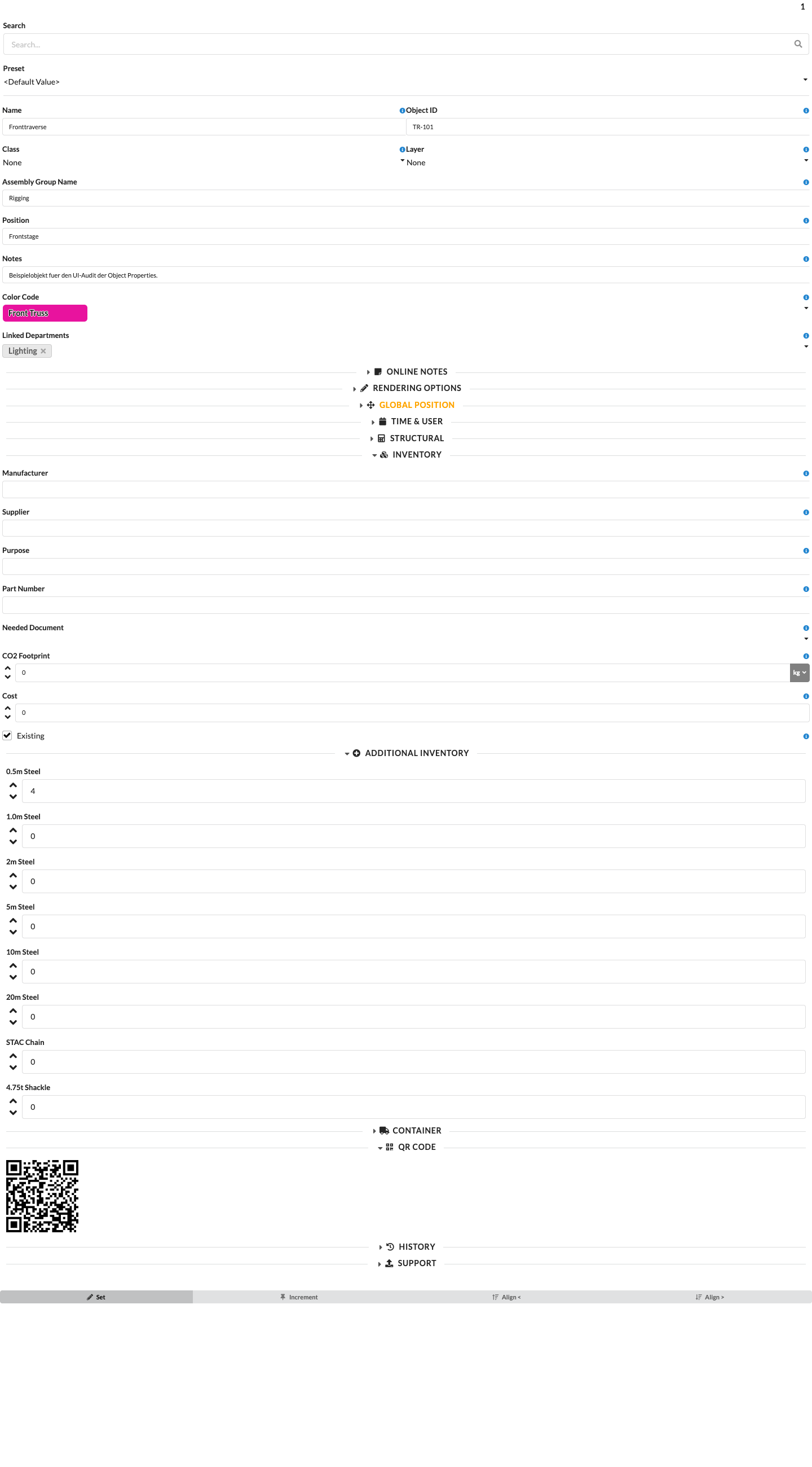
| Panel/Field | Detailed Description |
|---|---|
| [Inventory name] | Shows the stock for the respective inventory geometry, for example individual truss lengths or rigging hardware. You can adjust the quantity for the object. |
When an individual inventory object is selected, its stock and geometry data are also shown.
| Panel/Field | Detailed Description |
|---|---|
| Count | Sets how many items of this type are available. |
| Length | Gives the length of the inventory object, for example a cable, beam, or pipe. |
| Minimum Length / Maximum Length | Set the permitted length range for the object. |
| Length Difference | Gives the permitted difference between inventory lengths. |
| Cross-Sectional Area | Gives the conductor cross-sectional area for cable inventory. |
| Insulation Material | Selects the insulation material for the cable geometry, such as H07RN-F, PVC Multicore, SOOW, or SJOOW. |
| Inventory Type | Assigns the inventory object to a type such as Standard, Cable, or Bridle Part. |
| Color Code | Assigns an existing color code to the inventory geometry. The supplied Bridle parts already have defaults, which you can replace here. The Bridle View explains the color assignment and shows the color on the part and in its drawing labels. Color code names remain visible in the library and parts lists and are omitted only in drawing labels and their SVG export. The defaults use more distinguishable colors; saved colors and names are retained unchanged when loaded. Multicolor codes are displayed as color bands. |
| Weight in Structural | Mass of a complete Bridle component. A positive value is used directly. For steel ropes, 0 uses the mass calculated from the material length and selected rope definition. Standard hardware has editable numeric weights in grams; the defaults are listed in the Bridle View. Notes remain empty when created. Saved values, including 0, are retained unchanged when loaded. Other hardware without an entered mass remains incomplete. |
| Component WLL | Load capacity of the Bridle inventory part in the selected weight unit. For steel ropes, a positive value also limits the calculated rope load capacity; 0 uses only the rope definition. Standard shackles use 4,750 kg, STAC parts 5,400 kg, and the standard chain shortener a reference WLL of 5,300 kg. The defaults apply when created; saved values, including 0, are retained unchanged. For other hardware or an explicitly removed standard rating, 0 means that no rating is available. |
| Rope safety factor / Termination efficiency (0–1) | For rope inventory parts, editable factors for converting minimum breaking force into rope load capacity. Starting values: 5 and 0.9; adjust them to the actual application and termination. Details and the calculation basis are given in the Bridle View. |
You can also edit Bridle material sets directly using Edit Bridle… → Bridle configuration → Edit material set…. There you can add and remove local Bridle inventory geometries and change names, color codes, dimensions, and component values. Save material set updates all Bridles in the current drawing that use the set, including manual assignments and hidden entries. Removed or disabled parts are removed from assignments; automatic legs are reassembled. Open part previews must first be applied or discarded. Details about saving, undoing, and missing parts are provided under Edit Material Sets in the Bridle Dialog.
More about creating and editing symbols is available under Symbol Workflow. | Inventory Type | Assigns the inventory object a type such as Standard, Cable, or Bridle Part. |
For more about creating and editing symbols, see Symbol Workflow.
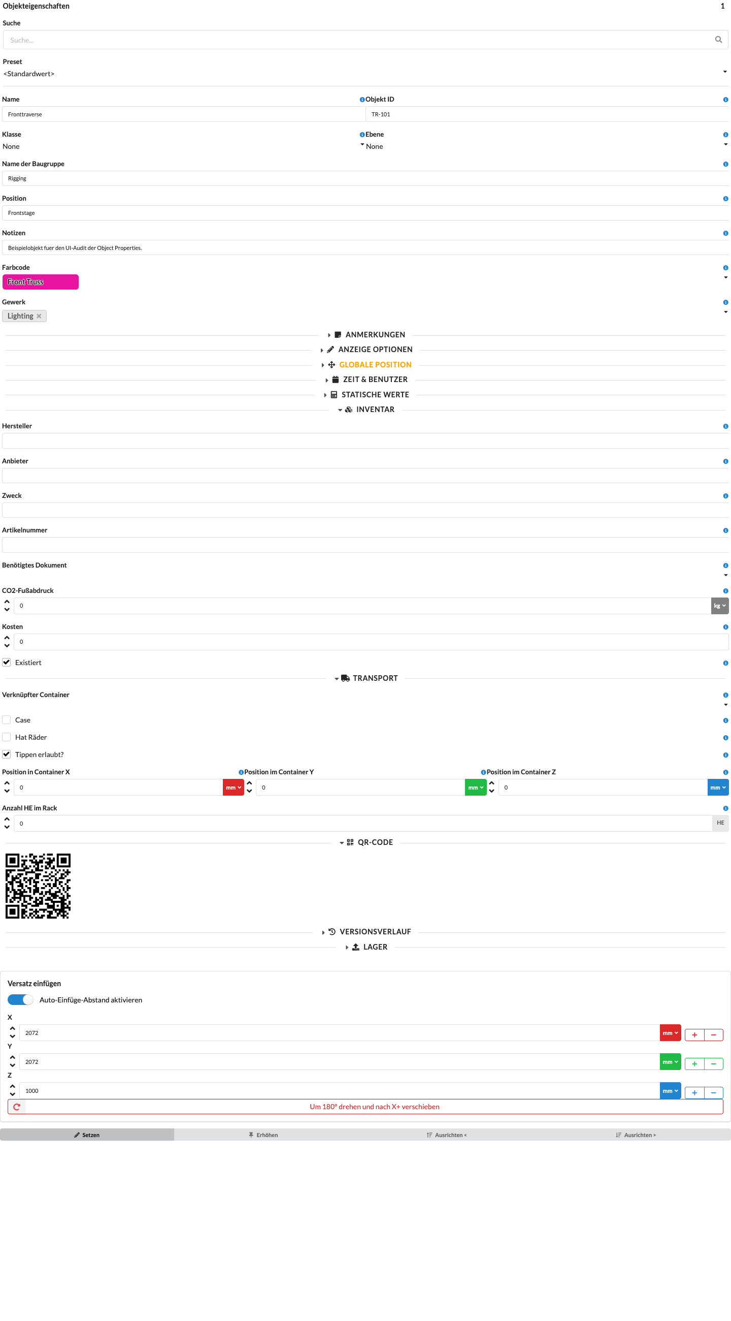
You can also enter important information for truck planning here, such as pack size, rack height, or the truck, case, or rack into which an object is packed.
There are four ways to pack objects:
Under Linked Container, you can select trucks, cases, and racks created earlier in Navigation. The Racks and Trucks sections there explain the container types.
| Panel/Field | Detailed Description |
|---|---|
| Linked Case Template | Selects a case template for planning a new case. |
| Linked Container | Specifies which truck, case, or rack the object is assigned to, integrating it directly into transport planning. |
| Position in Rack | Sets the rack unit at which the object is placed. |
| Case | Indicates that the object has its own case, so Production Assist treats it as a packed unit rather than a loose item. |
| Has Wheels | Indicates whether the object or case has wheels. This can affect packing logic, handling, and space requirements. |
| Allow Tip? | Allows the object to be tipped while packing or loading. This matters when material may or may not be transported in a rotated position. |
| Position in Container X, Y, Z | Shows the calculated position of the object within the container so you can see where it is placed in the packing volume. |
| Case Size X, Y, Z | Sets the width, depth, and height of the case or packing volume. |
| Rotation in Container X, Y, Z | Shows the calculated orientation of the object within the container around the three axes. |
| Count in HE Rack | Sets the rack units the object requires, which is especially important when planning equipment in 19-inch racks. |
To pack an object in a rack, first assign it a rack height. A case must have enough free slots for the object.
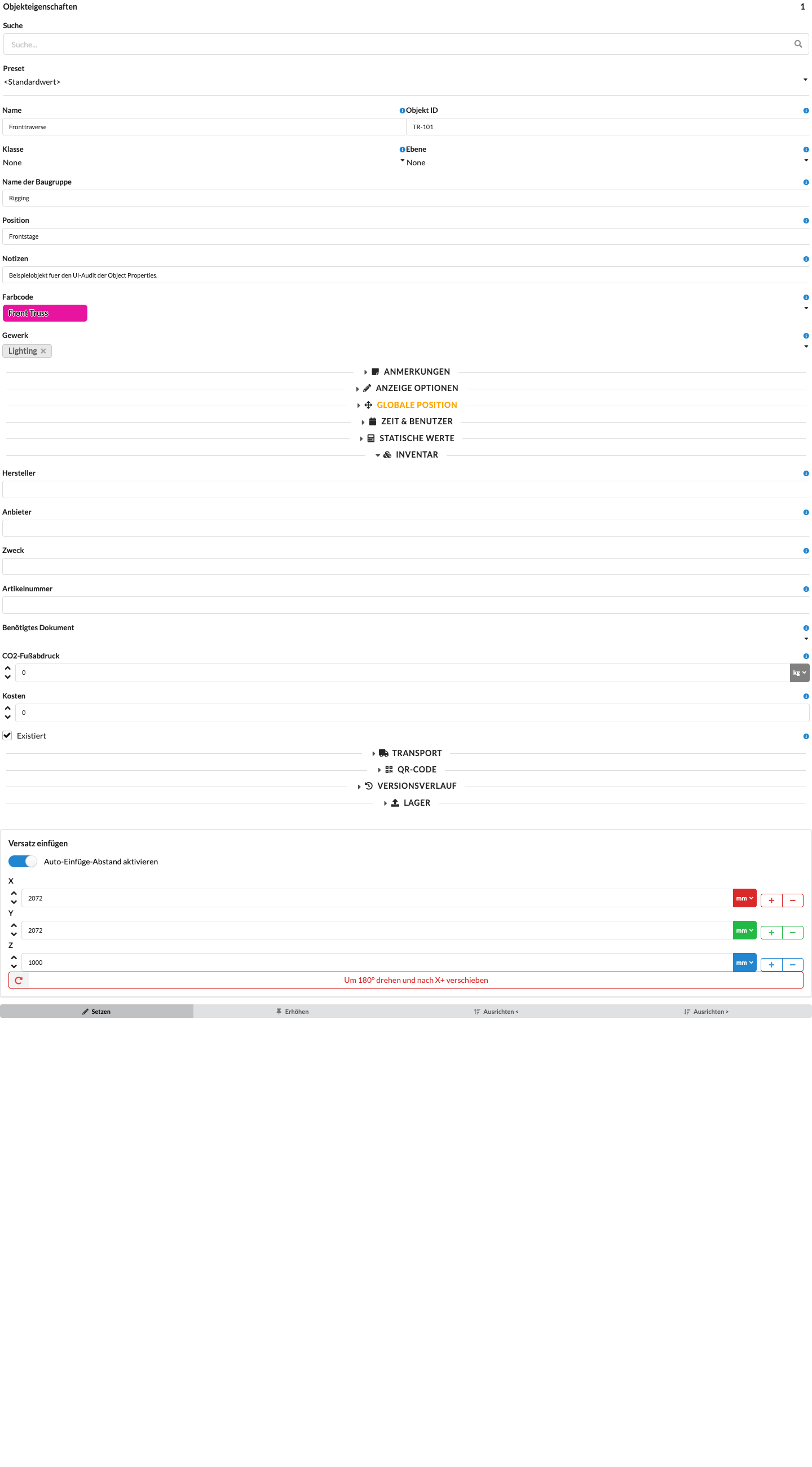
The QR code shown here links to the online address of the selected object. Whether other people can open its page depends on whether the project is available online and which access rights or sharing permissions apply. For labels, you can add a custom QR Code field that links to the object page in the online project. These links do not work without an online project; the example image uses a synthetic project address. For more information, see Create and Print Labels, Share a Project Link and QR Code, and the QR Code Workflow.
| Panel/Field | Detailed Description |
|---|---|
| QR Code | Links to the online address of the selected object. The object page is accessible only if the project is available online and the person scanning the code has the required access rights or a suitable sharing link. |
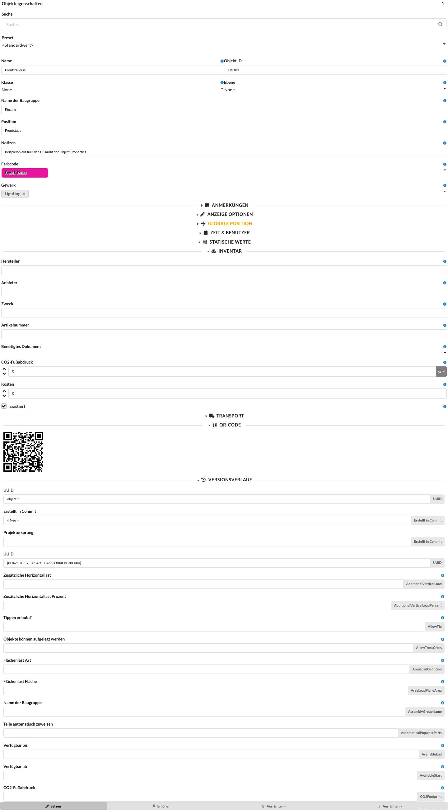
In the Version History panel, you can see which saved change state an object comes from. This lets you trace which changes to the object were documented most recently. It is similar to change tracking: this panel is usually not important for day-to-day planning, but it is very helpful when tracing changes.
| Panel/Field | Detailed Description |
|---|---|
| UUID | Shows the unique identifier of the most recently documented change state. This field is mainly relevant for technical tracking and helps identify changes unambiguously. |
| Creation ID | Shows the identifier under which the object was originally created. This makes it possible to trace the origin of this object. |
| Project Origin | Shows which project or data source the saved state was taken from. This is useful when content has been copied or synchronized from other projects. |
| Other fields in the panel | Depending on the object, additional saved properties appear below, such as Additional Horizontal Load, Allow Tip?, or Assembly Group Name. These values help you better understand earlier states of an object. |
The list is long and scrollable; the image shows an excerpt of the available version data.
For objects with a defined path, the Object Path panel appears after the Inventory panel. It shows the selected path point, the number of points, and the total length. Use the coordinate fields to edit the position of the selected point.
| Panel/Field | Detailed Description |
|---|---|
| Select Point | Switches between the points of the object path. |
| Number of Points | Shows the total number of path points. |
| Total Length | Shows the calculated length of the complete object path. |
| X, Y, Z | Edit the coordinates of the selected path point. |
Fixture Data includes all parameters related to the data planning of fixtures.
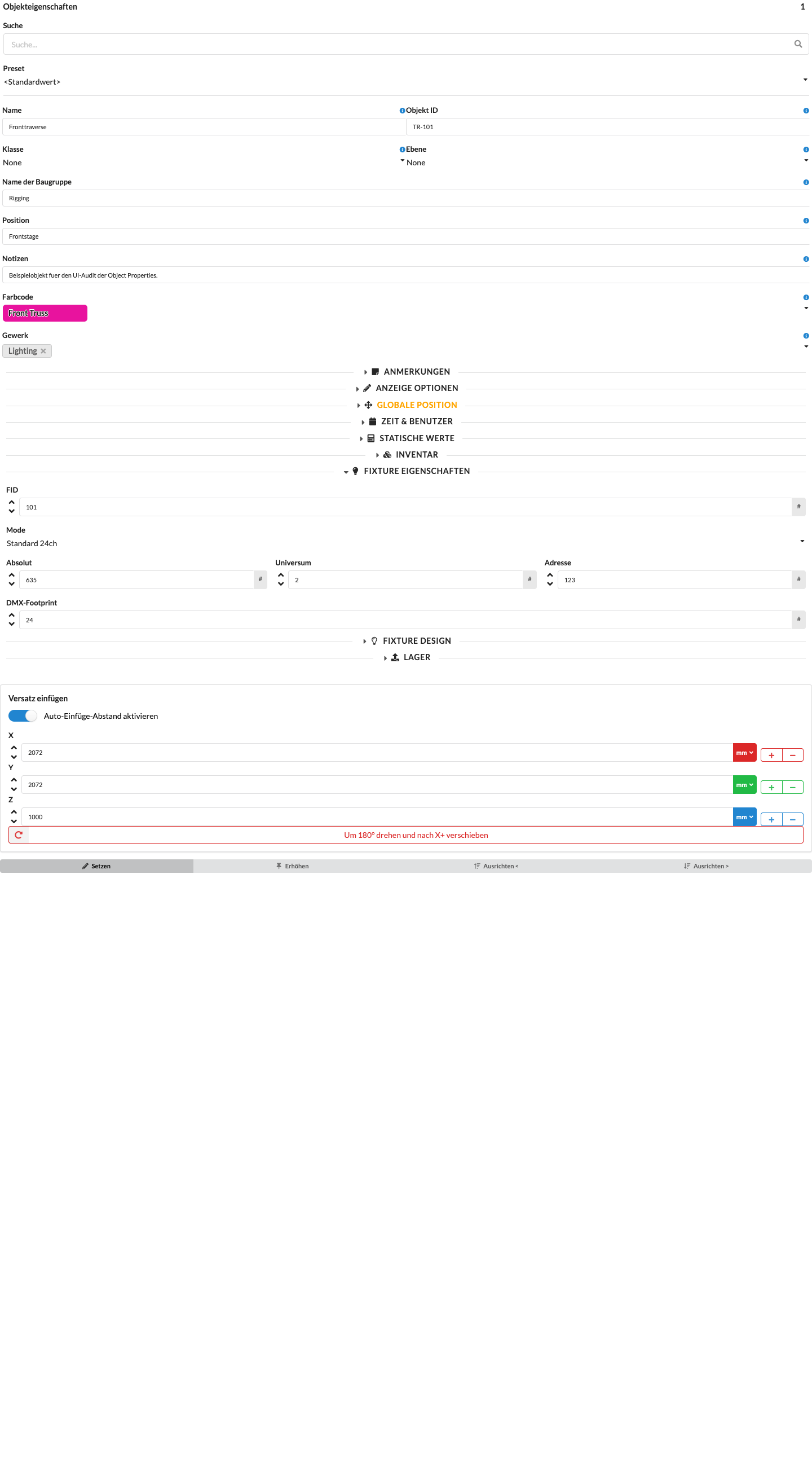
| Panel/Field | Detailed Description |
|---|---|
| Fixture ID | Sets the fixture's numeric identifier. It is used for unique assignment, appears in the Scene Tree, and is used to address the fixture on a lighting console. If the Object ID is empty or numeric, it is adjusted to match when the Fixture ID is changed. |
| Mode | Sets the operating mode used by the fixture. This determines which functions and how many DMX channels the device uses. |
| Footprint | Shows the number of occupied DMX channels. This value is usually taken automatically from the selected mode. |
| Absolute | Shows the absolute DMX address across all universes. This makes it easier to check larger patches. |
| Universe | Sets the DMX universe in which the fixture is patched. |
| Address | Sets the fixture's start address within the selected universe. |
The Fixture ID is the numeric identifier that also appears before the name in the Scene Tree. If the Object ID is empty or consists only of a number, Production Assist copies the Fixture ID value to the Object ID when you change the Fixture ID. An existing nonnumeric Object ID is retained. If the Fixture ID is red, it has been assigned more than once in the plan.
Under Mode, select the appropriate operating mode. The displayed DMX Footprint is taken from the selected mode. If the mode is missing, click the Mode field, enter its name, and select the suggested Add entry. Press Enter to open the Add New DMX Mode dialog. A fixture with an editable Mode field must be selected.
| Panel/Field | Detailed Description |
|---|---|
| Mode Input | Enter the name of the new mode if it is not yet in the list. |
| Add | Select the Add suggestion for the entered name and press Enter to open the creation dialog. |
In the Add New DMX Mode dialog, set the name and up to four DMX footprints. Use the channel counts from the fixture manufacturer's data. The four footprint fields start at 0; enter values only for the DMX breaks that are present. The Renderer does not currently contain a matching German audit render for this dialog. The following image therefore shows only an older English UI version and does not establish the current labels.
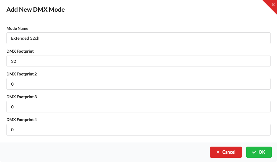
| Dialog/Field | Detailed Description |
|---|---|
| Mode Name | Sets the name that can then be selected in the Mode field. |
| DMX Footprint | Gives the number of DMX channels for the first DMX break in this mode. |
| DMX Footprint 2–4 | Enter channel counts for additional DMX breaks if the fixture uses them. The four input fields default to 0. |
| OK | Creates the mode for the Fixture Type, sets it as current, and closes the dialog. The footprint values are saved with the mode. |
| Cancel | Closes the dialog without creating the new mode. |
Enter the footprint channel counts from the manufacturer's data. After selecting OK, check that the new mode appears in the Mode field and that DMX addressing matches the device. The dialog has numeric fields but does not show documented range validation or instructions for invalid footprint values. Refer to the fixture documentation.
Under Universe and Address, enter the universe and fixture start address. Production Assist calculates Absolute, the sequential address across all universes, from these values. If the relative address is greater than 512, a warning appears; you can cancel or continue with Continue.
For more ways to patch fixtures, see the local tutorial Create Power and Network Patch Worksheets.
Fixture Design contains all parameters that are important for lighting design.
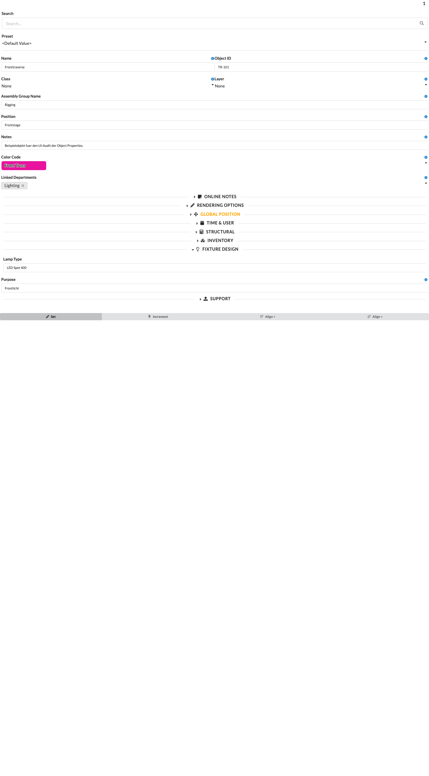
| Panel/Field | Detailed Description |
|---|---|
| Lamp Type | Shows or sets the lamp type for the fixture. This information is also used later in the Paperwork. |
| Purpose | Describes what the fixture is used for, for example key light, backlight, or an effect. |
| Dimmer Intensity | Controls the brightness of the light output in the Renderer, allowing you to adjust the fixture's visual effect. |
| Lamp Rotation | Rotates the fixture's representation, for example from a hanging to a standing position. |
| Beam Angle / Field Angle | Set the size and spread of the light beam. This lets you match the lighting effect in the Renderer more closely to reality. |
| Frame Size | Stores the required frame size for Paperwork and accessory planning. |
| Light Color | Shows the selected light color and opens the color dialog when needed. |
| Filter / Gobo / Pan / Tilt | This panel contains other design parameters for controlling the fixture's appearance and orientation in the Renderer. |
For a simple symbol, you can only enter the lamp type for later use in the Paperwork.
For a GDTF fixture, additional parameters are shown. The GDTF fills them in automatically, but you can also change them. They always affect the fixture's appearance in the Renderer.
Enter the lamp's intended use primarily for later use in the Paperwork.
Use this setting to control the spotlight's light output in the Renderer. To make a light beam visible, choose Fast or Beautiful for Spotlight Beam Display under File → Settings... → Renderer. Off hides the light beam.
Lamp Rotation lets you turn hanging spotlights into standing spotlights by rotating them 180°.
These two fields control the size of the light beam.
The Frame Size is used later in the Paperwork to calculate the number of required gel cuts and rolls.
You can change the beam color here. Click the pencil icon to open the Choose a Color dialog. When opened from Object Properties, the field name is not added to the dialog title. The Color Picker uses the CIE color system. You can set a color in four ways:
Black and white are available as quick selections. The Light Color field must be available in the selected object's Fixture Design section. OK applies the selected color to the object; Cancel closes the dialog without applying an unconfirmed selection. The beam color is visible in the Renderer only when Spotlight Beam Display is set to Fast or Beautiful under File → Settings... → Renderer; Off hides the light beam.
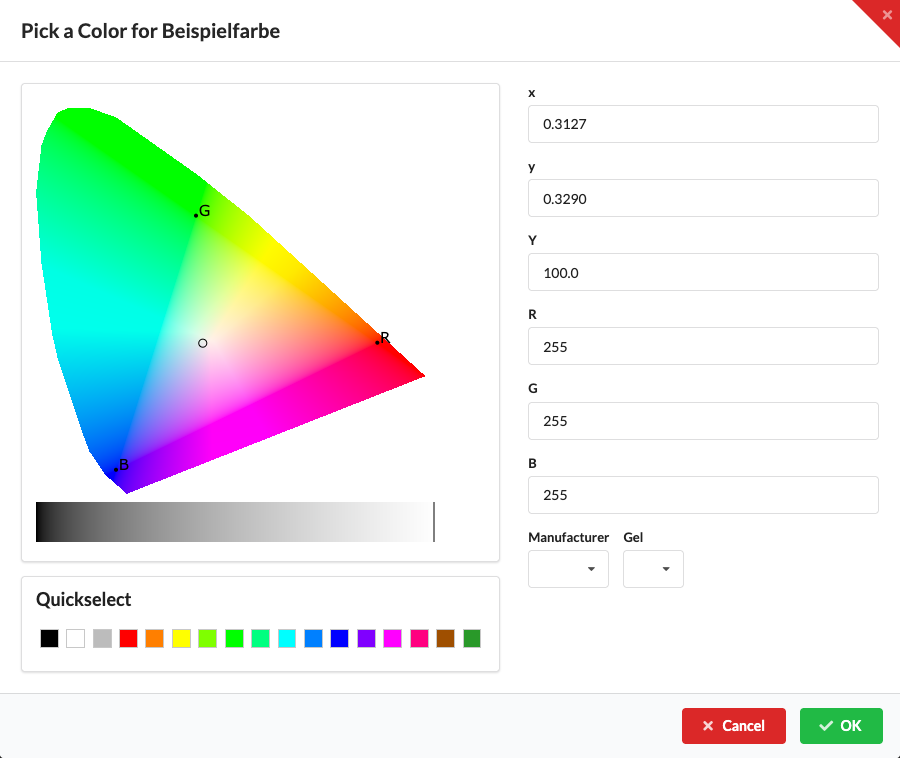
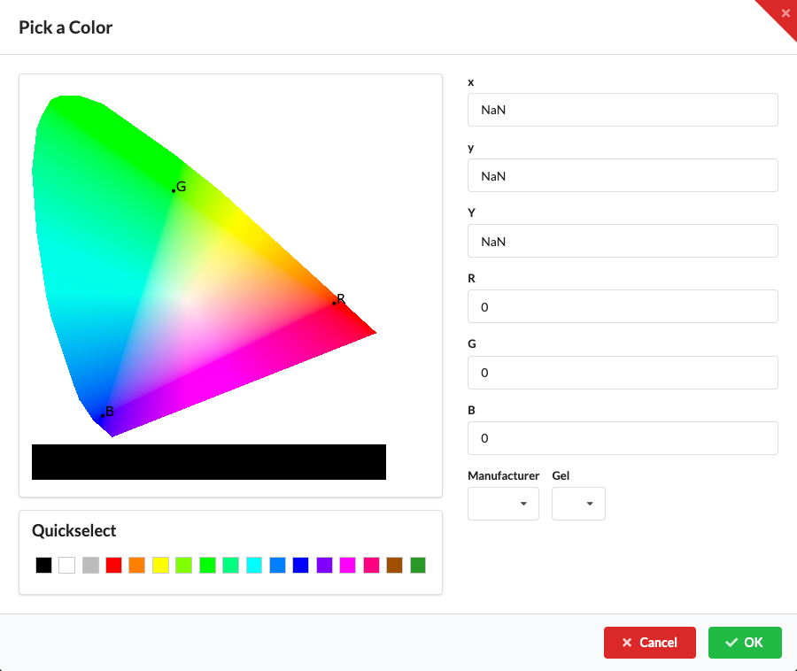
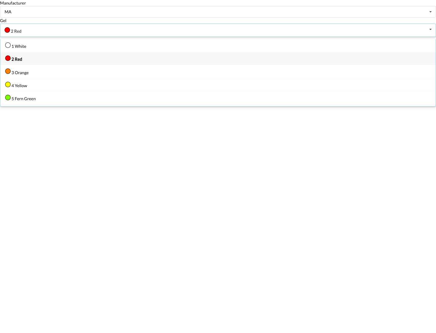
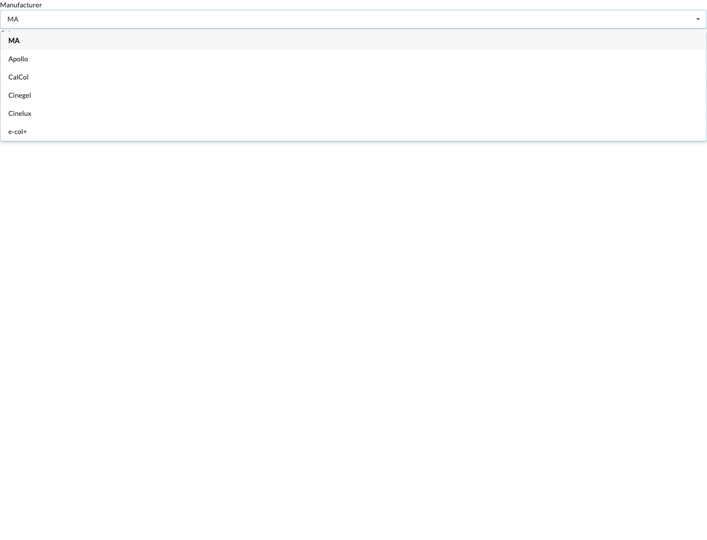
The x and y fields specify the color location in the CIE color system, and Y specifies brightness. R, g, and B specify the red, green, and blue components. The two input methods are converted into one another. Select a manufacturer first, then the appropriate color filter; the two open lists are shown separately above. OK applies the selection; Cancel discards it.
| Dialog/Field | Detailed Description |
|---|---|
| Color Field | Select the desired color visually here. This helps you quickly find a suitable color impression. |
| Brightness Slider | Adjusts the brightness of the selected color, so you can make the same hue lighter or darker. |
| CIE Values | Enter exact color coordinates in the CIE color system in these fields. This is useful for standardized or reproducible colors. |
| RGB Values | Set the color using numeric RGB values. This is useful when applying precise screen or corporate identity colors. |
| Gel Selection | Lets you select a manufacturer and a specific color gel so you can use real filter materials in the plan. |
| Black/White Quick Selection | Quickly selects black or white without entering values manually. |
After you confirm with OK, both the beam in the Renderer and the Light Color field display the corresponding color. The field also shows the color-space coordinates.
The color field in the object palette shows the current color value. Click the pencil icon to reopen the color dialog and adjust the color later.
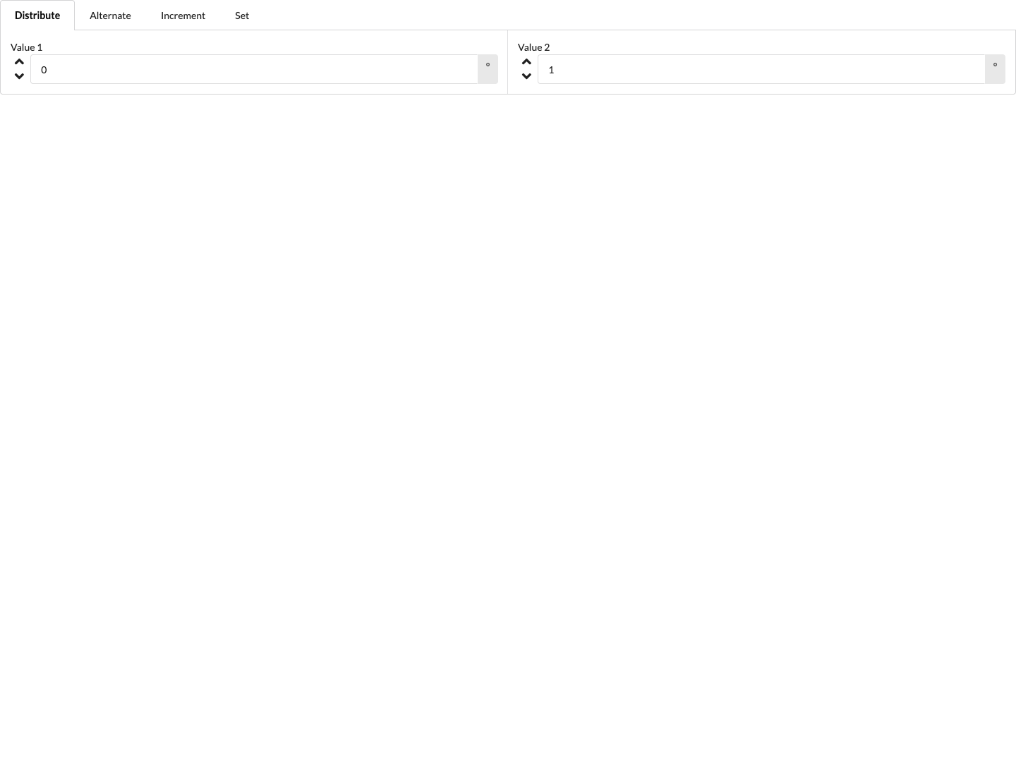
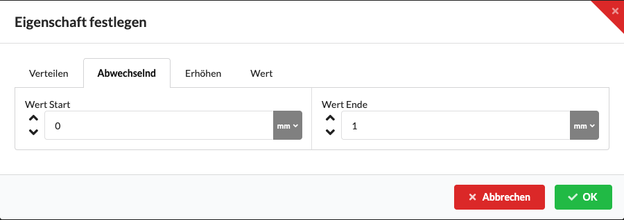
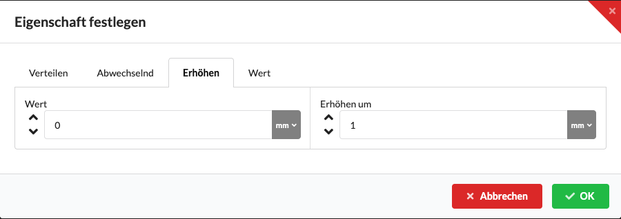
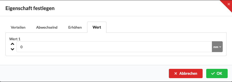
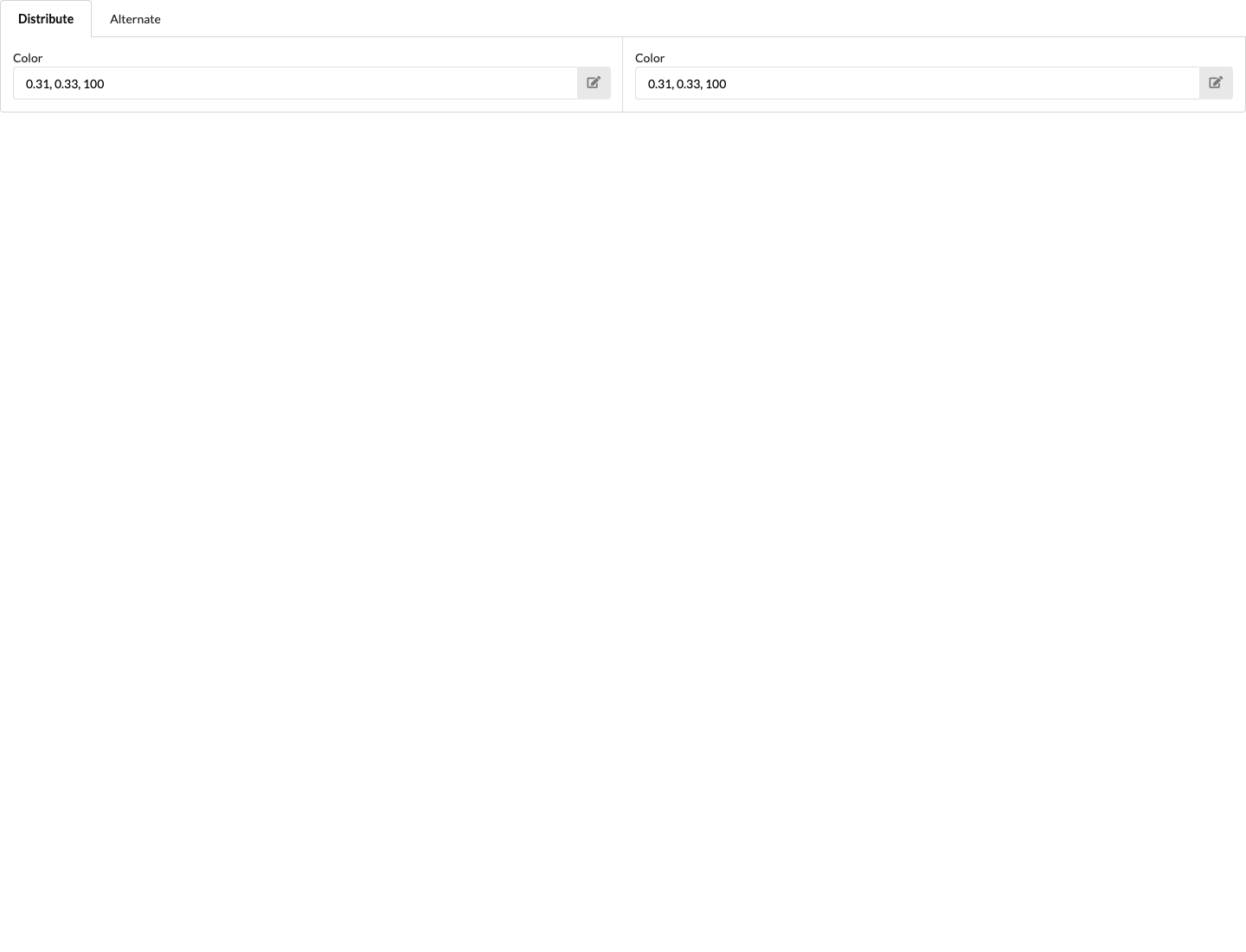
When multiple objects are selected, clicking the label of a numeric field in Object Properties opens the Set Property dialog. For Light Color, open it using the chart icon next to the color field. Select one of the four tabs to choose how the property is applied to the selected objects. Enter numeric values in the displayed unit. OK applies the values to the selection; Cancel closes the dialog without applying them. Then check the result on the selected objects. There is no separate input view for text fields.
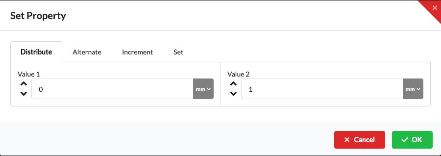
The compact image shows the numeric input area of the same dialog in Distribute mode:
The following images show the other tabs in the full dialog:
| Mode | Use |
|---|---|
| Distribute | Set the start and end values with Value 1 and Value 2. Production Assist distributes the values evenly across the selected objects. For example, use this mode to give a row of objects gradually changing position or angle values. |
| Alternate | Set two values with Start Value and End Value. The selected objects alternate between them. This works for a repeating pattern, such as alternating heights or angles. |
| Increment | Enter the starting value under Value and the step under Increment by. This lets you increase or decrease the value in equal steps across the selection. |
| Value | This tab provides a single numeric field for a shared value. Currently, this mode does not reliably set a uniform numeric value. If needed, change the field directly in Object Properties. |
For Light Color, the Distribute and Alternate modes are available. In both tabs, select two colors: Distribute grades the colors across the selected fixtures, while Alternate switches between them.
Under Manufacturer, you can select a gel manufacturer, and under Gel, the appropriate filter gel. This is used later in the Paperwork to determine the number of required gel cuts and rolls.
If gobos are stored in the GDTF, you can select them here. They will then be visible in the Renderer.
Throw Distance is a read-only, automatically calculated value. It shows the length of the light path from the beam to ground level, so it depends on the fixture's position and orientation. If the beam points horizontally, Production Assist cannot calculate an intersection with the ground plane.
Use Pan and Tilt to pan and tilt the spotlight in the Renderer.
This section appears when your selected object has electrical or network-based connections. Here, you plan both power and data cabling.
The complete manual and automatic patching workflow is described under Electrical Planning.
This panel contains the object's electrical connections. The first section covers the power connection. Here you can find the selected object's Input and Output connections, their Connector type, and the required Power. Once cabling is complete, the main connection supplying power is also displayed. You can also enter a cable length for paperwork.
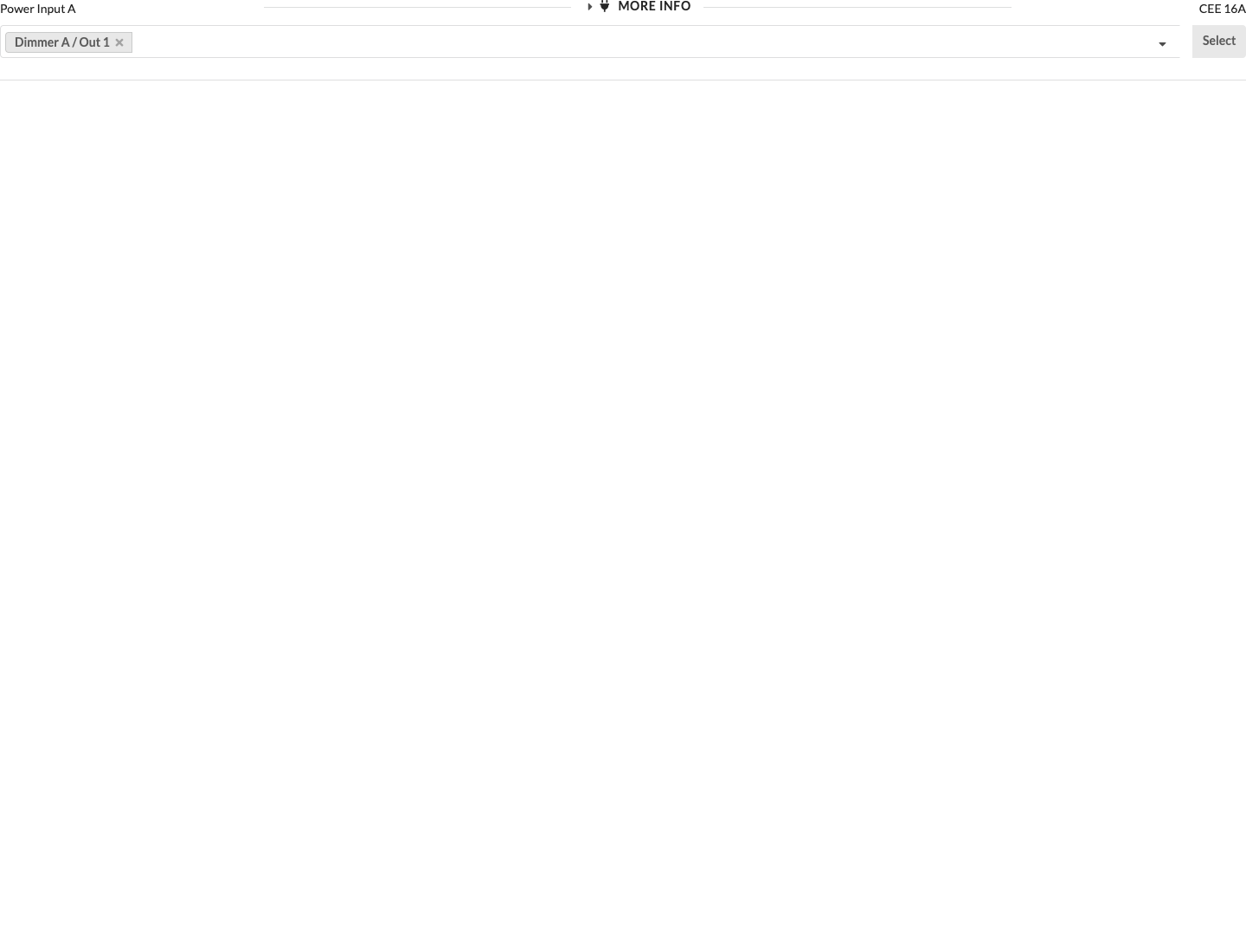
| Panel/Field | Detailed Description |
|---|---|
| Mark as Fully Connected | Marks all of the object's connections as fully connected, even if some connections are still free. This is useful for marking placeholders as complete or green so that open connections can be used specifically later. |
| Preliminary Mains Connection | Sets a preferred power source for the object. This lets you prepare the later power feed and determine the power load before the object is fully patched. |
| Available From / Available Until | Limits a generator object's availability to the specified period. These date fields appear for generators. |
| Input | Shows the object's input or outputs. Here you can see directly which connections can be patched or checked. |
| More Info | Opens or closes the additional details for this connection. These include power values, phase loading, and cabling. |
| Patch Field | Sets the device or connection to patch to. You can also search in this field by typing. |
| Select Button | Jumps directly to the selected counterpart object or distributor. This is useful when you want to continue working on the cabling there. |
To connect the selected object to another device:
A check mark before an entry indicates that the connection is already in use. Check its existing connection before selecting it as well. This selection list does not provide an automatic prompt to replace the connection.
After a successful selection, the connection is linked to the selected counterpart object. You can see this because the entry appears in the Patch field, and you can jump directly to the connected object using Select.
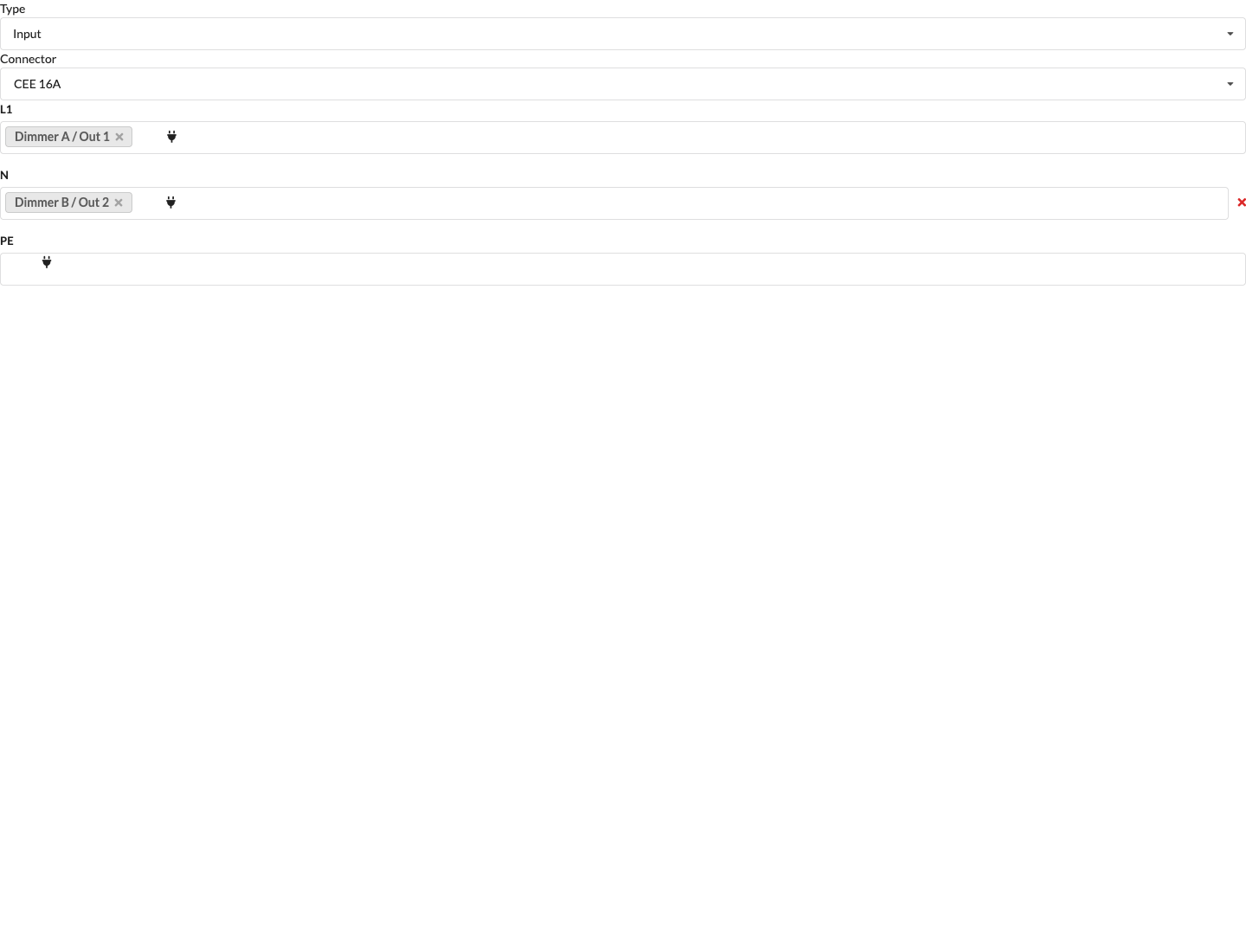
| Panel/Field | Detailed Description |
|---|---|
| Patch List | The screenshot shows the list of available connections on a consumer. Select the distributor or connection from which the object should receive power. |
| Search Field | Type in the panel to find available connections more quickly. This saves time, especially in large projects with many distributors. |
| Status Indicator | The indicator before the name identifies devices that are already patched. This lets you see immediately whether a connection is occupied. |
Note: To limit manual connection selection to the Assembly Group of the object you are editing, enable Limit patch options to local group under File → Settings... → Electrical.
If you want to define power distribution for the following fixtures directly through a distributor (for example, the selected plugbox), you can activate the distributor in the Scene Tree or, if you have just connected a fixture to it, click Select to the right of the drop-down menu. This takes you to the selected distributor, where you can select the desired fixtures for its remaining free outputs.
| Panel/Field | Detailed Description |
|---|---|
| Output List | The screenshot shows the open panel on a distributor. Set which consumer is connected to each output here. |
| Occupied and Free Outputs | You can see directly which outputs are still free and which are already in use. This makes it easier to distribute consumers clearly. |
| Continue Working at the Distributor | This view is especially useful when you want to patch several subsequent devices to the same distributor one after another. |
The additional panels help you check power connections correctly and plan suitable cables.
| Panel/Field | Detailed Description |
|---|---|
| Input | Shows the input currently being viewed, making clear which connection the following details refer to. |
| Mains Connection | Shows which mains connection is assigned to this connection. The row appears when a mains connection is linked. |
| Power | Shows the object's current power. This value helps you assess the actual load. |
| Maximum Power | Shows the maximum available or permissible power at this connection, so you can see whether capacity remains. |
| Phase Loading | Opens or closes the phase loading values. These values help identify imbalanced loads or overloads early. |
| Cabling | Opens or closes the cable values for this connection. Here you can check cable lengths, cable types, and manual cable selection. |
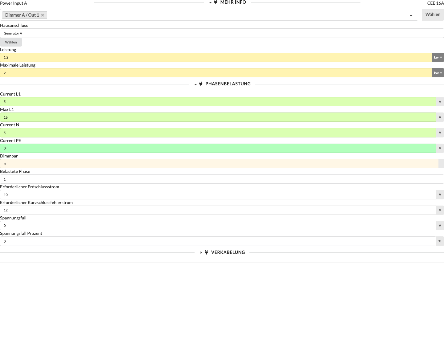
| Panel/Field | Detailed Description |
|---|---|
| Current L1, Current L2, Current L3 | Show the current drawn on each phase. Use these values to see how evenly the load is distributed across the three phases. |
| Max L1, Max L2, Max L3 | Show the maximum permitted current on each phase. These values help you avoid overloads. |
| Current N | Shows the current on the neutral conductor. This value matters when loads are unbalanced. |
| Current PE | Shows the current on the protective conductor. This display is primarily for technical checks. |
| Loaded Phase | Shows which phase the connection loads. This makes it easier to assess the phase assignment. |
| Required Earth-Fault Current | Shows the required earth-fault current for protection. This value supports the technical assessment of the connection. |
| Required Short-Circuit Fault Current | Shows the required short-circuit fault current for the design. This value also supports a technical check of the power supply. |
| Voltage Drop | Shows the voltage drop in volts, so you can see whether cable lengths or loads cause significant losses. |
| Voltage Drop Percent | Shows the voltage drop as a percentage, making it easier to compare against permitted limits. |
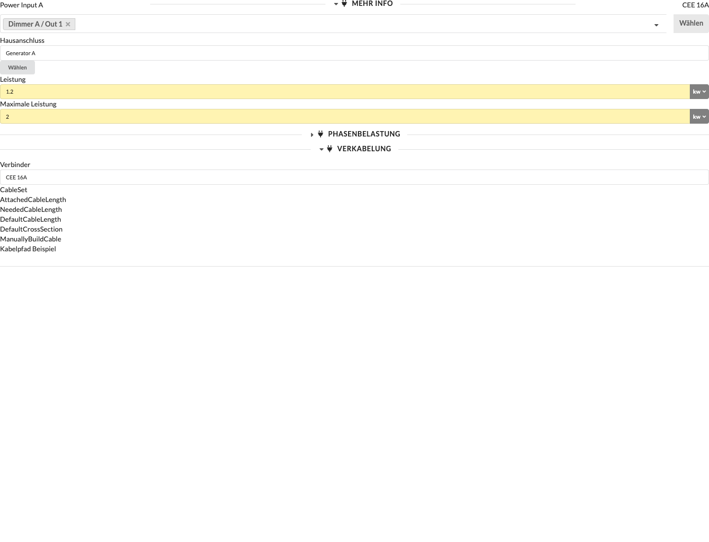
| Panel/Field | Detailed Description |
|---|---|
| Connector Type | Shows the connector type used by the connection, making it clear which cables are technically suitable. |
| Cable Set | Selects the cable set from which suitable cables are drawn. This is useful when working with different cable inventories or standards. |
| Cable Length | Shows the cable length assigned to this connection. This value is generated automatically and serves as a planning basis for the connection. |
| Required Cable Length | Shows the automatically calculated required cable length. It is based on the ideal distance between the devices along the cable path. |
| Standard Cable Length | Sets the standard cable length for automatic assignments. This speeds up cable planning for recurring cases. |
| Standard Cable Cross-Section | Sets the cable's standard cross-section. This matters for technical suitability and voltage drop. |
| Assemble Cable Manually | Enables manual cable assembly, allowing you to depart from the automatic logic when needed. |
| Name | Shows the available cable types in the list. Select the specific cable assembly from this list. |
| Count | Increases or decreases the quantity of the respective cable type, letting you specify exactly which cable combination to output. |
The second section covers data distribution. Here you can find the available Data Inputs and Outputs, the universe distributed at this connection, and the connection type.
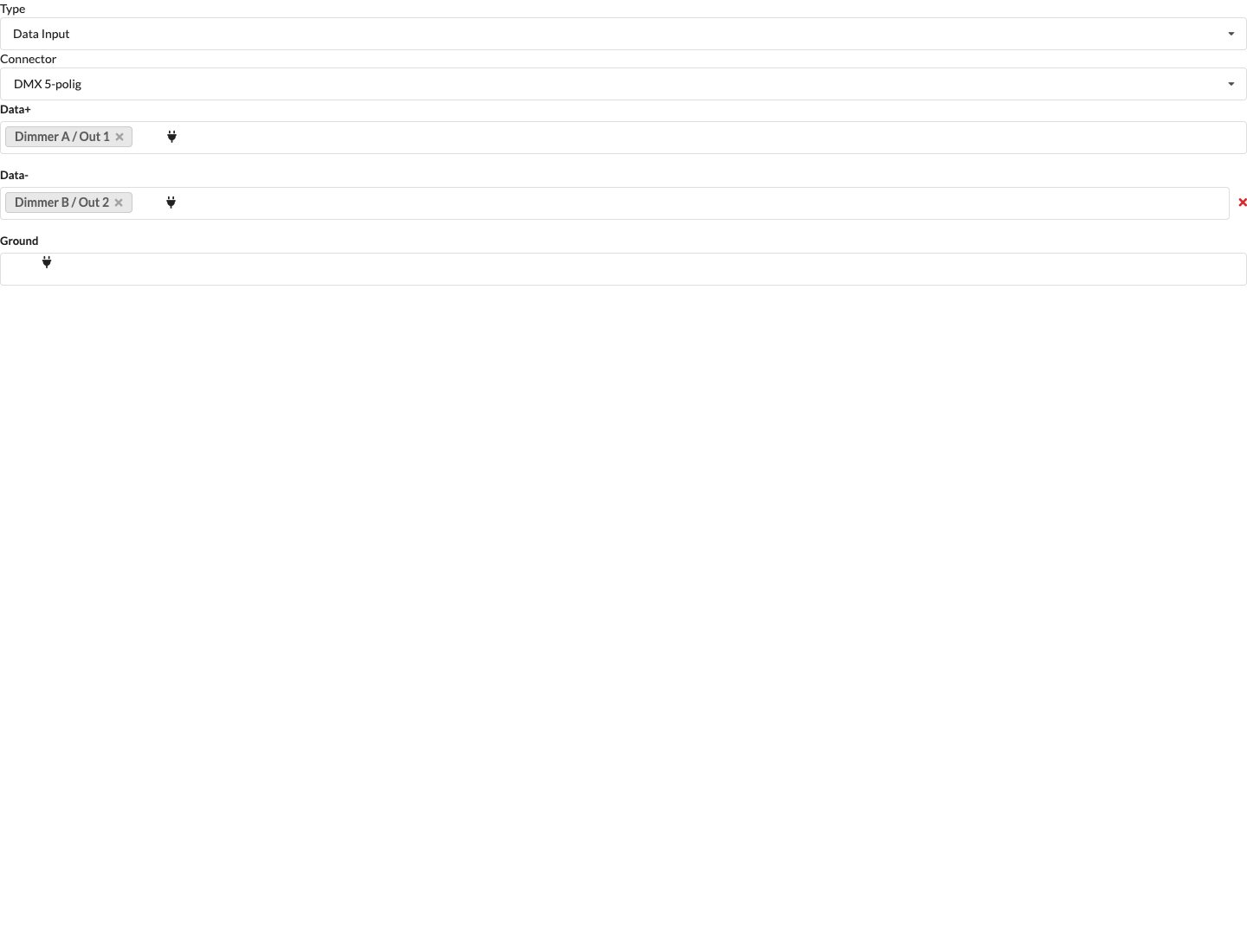
| Panel/Field | Detailed Description |
|---|---|
| Data Input / Data Output | Shows the selected object's available data connections. Plan here how data enters or passes through the object. |
| Universe Display | Shows which universe is distributed or expected at this connection. This helps you check the data structure. |
| Patch Field | Use this field to link the data connection to another device or distributor. |
| Select Button | Jumps directly to the linked counterpart object so you can continue editing the data path there. |
| Default Network Cable Length | Sets the default length for automatically planned network cables at this object. |
To connect the selected object to another device:
A check mark before an entry indicates that the connection is already in use. Check its existing connection before selecting it as well. To disconnect, remove the entry from the Patch field.
After a successful selection, the data connection is linked to the selected counterpart object. You can see this because the entry appears in the Patch field, and you can jump directly to the connected object using Select.
| Panel/Field | Detailed Description |
|---|---|
| Patch List | The screenshot shows the list of available data sources on a device that receives data. Set which distributor or device provides the signal. |
| Search Field | Type in the field to find suitable data sources more quickly. This is especially useful when many connections are available. |
| Status Indicator | Entries that are already occupied or connected are marked, helping you avoid accidental duplicate assignments. |
Note: To limit manual connection selection to the Assembly Group of the object you are editing, enable Limit patch options to local group under File → Settings... → Electrical.
If you want to define data distribution for the following fixtures directly through a distributor (for example, the selected data box), you can activate the distributor in the Scene Tree or, if you have just connected a fixture to it, click Select to the right of the drop-down menu. This takes you to the selected distributor, where you can select the desired fixtures for its remaining free outputs.
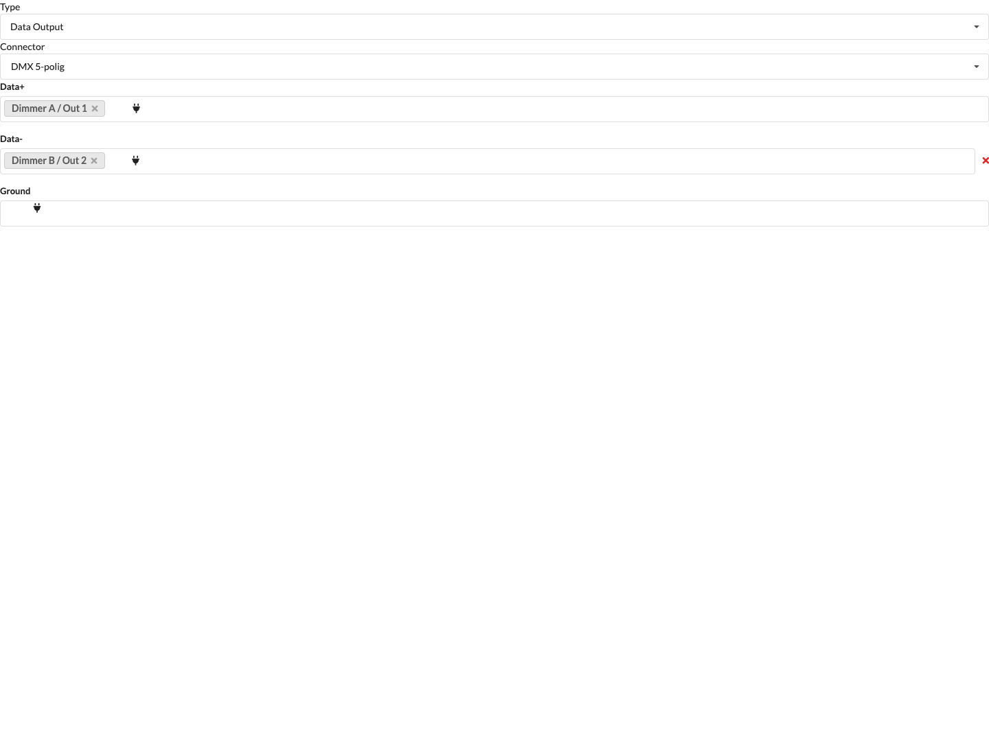
| Panel/Field | Detailed Description |
|---|---|
| Output List | The screenshot shows the open panel from a data distributor's perspective. Assign outputs directly to subsequent devices here. |
| Occupied and Free Data Paths | You can immediately see which outputs are still available and which are already in use. |
| Continue Working at the Distributor | This view is especially useful when you want to patch several devices to the same data distributor one after another. |
With Hotpatch, you manually assign selected devices to a distributor's hotpatch outputs. The matrix shows existing and free assignments, as well as power values and loads. A change is applied immediately; check the phase values afterward. The function does not automatically calculate an optimal distribution.
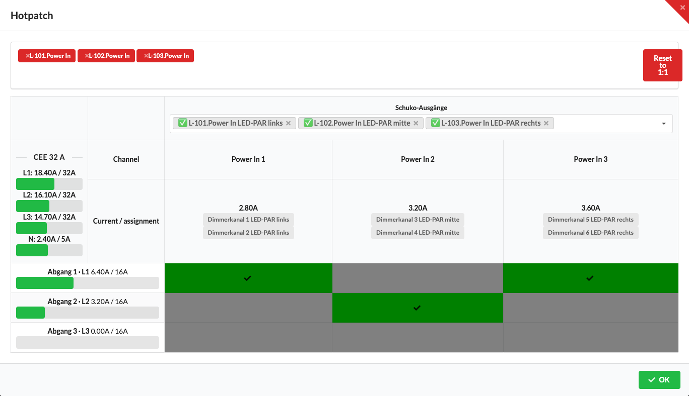
| Panel/Field | Detailed Description |
|---|---|
| Matrix | Rows show hotpatch outputs; columns show the hotpatch inputs of the selected devices. A check mark indicates an existing assignment. Click a cell to set or remove the assignment immediately. |
| Power Values and Load | Show the measured currents for the hotpatch outputs and connected inputs. Use them to check the effects of your manual assignment. |
| Reset to 1:1 | Restores the default assignment for the selection. It does not reconstruct an earlier hotpatch setup. |
| OK | Closes the matrix. |
Selected devices with suitable hotpatch inputs and outputs are required. For the steps, see Hotpatch in Electrical Planning.
For objects with electrical or network connections, such as fixtures, power connections, power distributors, or consoles, the icon color changes depending on how many connections are occupied:
| Color | Meaning |
|---|---|
| Red | All inputs/outputs are still unpatched/free. |
| Yellow | At least one input or output is connected, and others are free. |
| Green | All recorded inputs and outputs are connected, or Mark as Fully Connected is enabled. |
| Panel/Field | Detailed Description |
|---|---|
| Colored Icon in the Scene Tree | The icon before the object name shows the current patch status. In the tree view, you can see whether an object is still open, partially connected, or fully patched. |
| Assembly Group View | The status is shown directly on the icon in the Scene Tree. This makes it quicker to find open connections, even in larger Assembly Groups. |
This group appears for structural elements. It connects the geometry with cross-section and material data and provides permissible deformation and force values for structural calculation.
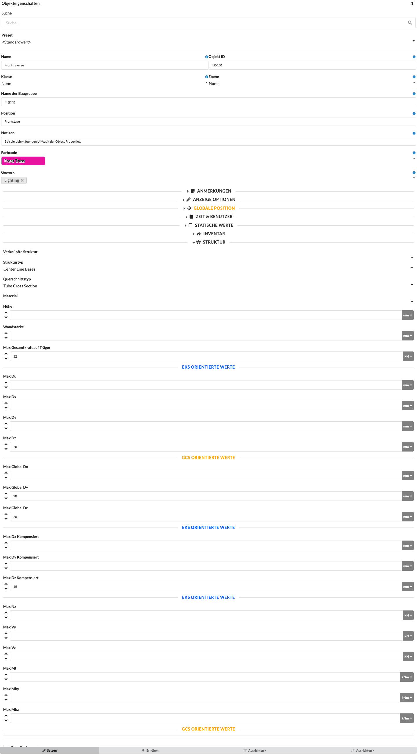
| Panel/Field | Detailed Description |
|---|---|
| Linked Structure | Assigns the element to an existing structure definition. |
| Structure Type | Selects the type of structural description, such as centerline or detailed geometry. |
| Cross-Section Type | Determines whether to use a truss cross-section, pipe, or rectangular profile. The following dimension fields depend on this selection. |
| Material | Sets the material for structural calculation. |
| Cross-Section | Selects the profile when using a template cross-section; for pipe and rectangular cross-sections, define height, width, and wall thickness in the corresponding fields. |
| Max. Point Load | Sets the permissible limit for a point load on this structural element. |
| Max. Deformation Du, Dx, Dy, Dz | Sets limits for resultant and axis-related deformations in the local reference system. |
| Global Deformation Limits | Sets limits for the global displacement components. |
| Local Forces Nx, Vy, Vz and Moments Mt, Mby, Mbz | Sets permissible limits for internal forces and moments in the local reference system. |
| Assign Cable Load | Controls whether cable loads can be assigned to this structural element. |
You see this section when you have selected a motor symbol or a symbol with a support point.
For simple symbols, the Name and the Support Name of the object are the same. However, if you have symbols that contain multiple support points, you can give each one a separate name here.
Here you will find information about chain length, load capacity, and speed. These values are important for the Paperwork and the structural calculation and can be changed here.
After a calculation has been performed, the load at the motor (Hook Force – without motor self-weight) and at the attachment point (Roof Force – including motor self-weight) is displayed here.
With Show Results in 3D, you can show or hide the results for the respective support in the 3D view. This setting does not change the calculation. For the label to appear, Show Labels in 3D must also be enabled in the global Renderer; see Renderer Settings.
If the motor is hung upside down, check this box.
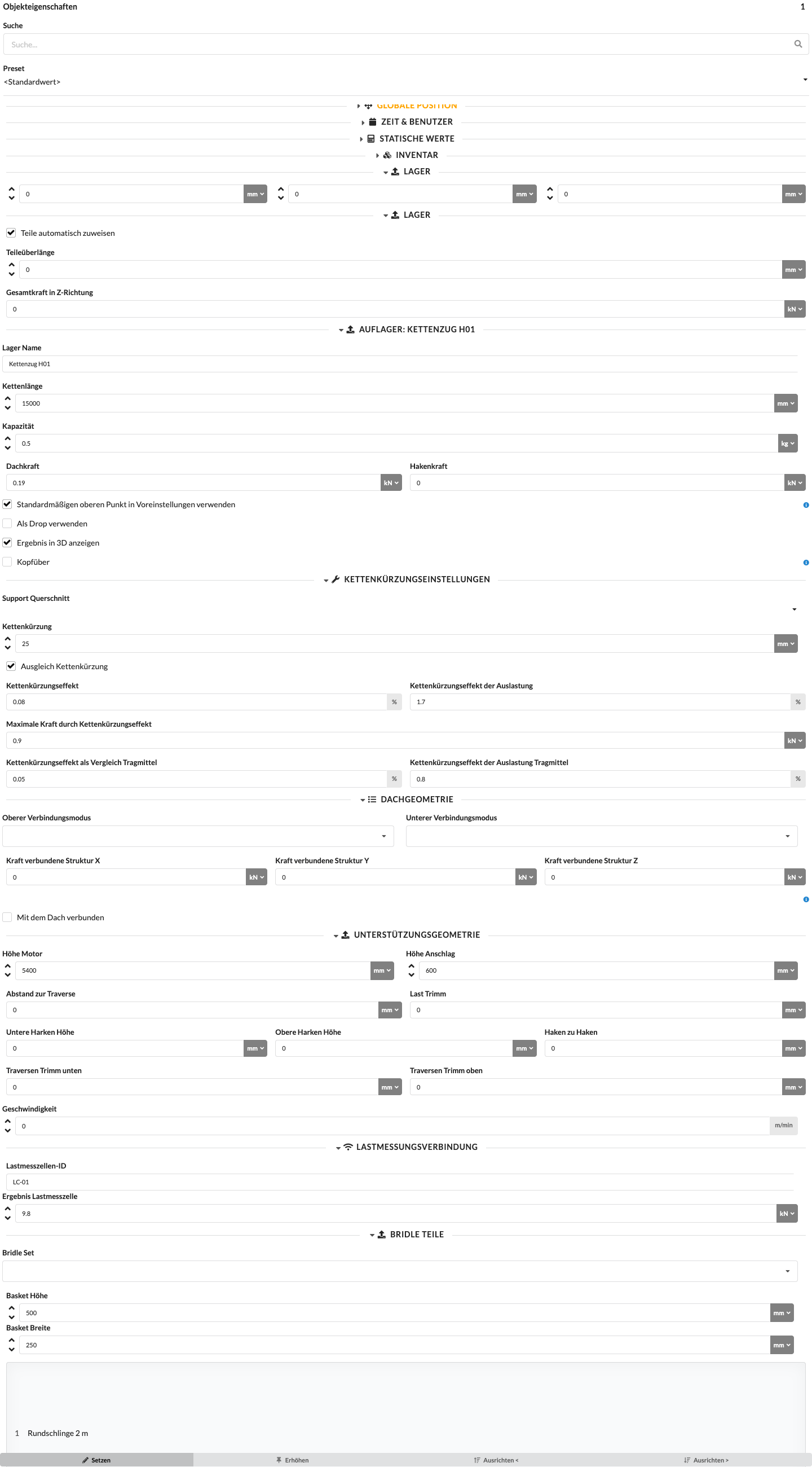
| Panel/Field | Detailed Description |
|---|---|
| Auto-Assign Parts | Searches for a combination of available rope and connection parts. For multi-leg bridles, it can connect shorter upper ropes to a drop. Attachment points and the load point remain fixed; any remaining length deviations are shown in the Bridle View. |
| Parts Excess Length | Shows the summed length differences of the assigned leg parts, including the basket. The value is updated when parts are applied, during automatic part assignment, and after saved geometry changes in the Bridle Builder. The individual signed deviations appear in the Bridle View. Differences in opposite directions can cancel each other out in the sum. |
| Total Force in Z Direction | Shows the total vertical force at the support. This value is important for assessing the load situation. |
| Support Name | Sets the name of the individual support. For symbols with multiple supports, each support can be named separately. |
| Chain Length | For rope and lifting-equipment supports, sets the rope or chain offset. This field may be read-only for automatically assembled multi-leg bridles. |
| Capacity | Sets the capacity for rope and lifting-equipment supports. For bridles with assigned parts, the smallest complete component capacity of the leg, including the basket and selected rope diameter, is used instead; the field is read-only there. Missing component values do not provide a complete capacity. After the calculation, compare the value with the displayed utilization. |
| Allow Uplift Forces | Allows the support to carry upward tensile forces. Disable this option for a compression-only support. |
| Rotated Support | Transfers the object's rotation to the FEM support so that it follows the inclined or rotated installation position. |
| Node Displacement X / Y / Z | Specifies a known displacement of the support node for the FEM calculation. The input does not move the attachment in the drawing. With finite support stiffness, the specified displacement produces a corresponding reaction. |
| Coefficient of Static Friction Between Ground and Support | Sets the coefficient of friction for the sliding safety check of a ground support. |
| Roof Force | Shows the force at the upper attachment point after calculation. This field is read-only. |
| Hook Force | Shows the force at the lower hook or lifting equipment after calculation. This field is read-only. |
| Use Default Upper Point in Presets | When placing this support, uses the upper connection point defined in the presets. This option is relevant when the upper connection point differs from the standard geometry. |
| Force Drop Connection | Treats this support as a drop. If it is not connected to a structure at the top, an error message appears. Check the message and the connection before using the calculation results. |
| Show Results in 3D | Shows or hides the calculation results in the 3D view so you can check them directly in the model. |
| Upside Down | For rope and lifting-equipment supports, determines where the self-weight is applied in the calculation. When enabled, the weight is applied at the upper node; otherwise, it is applied at the lower node. This setting affects only the calculation and does not change the 3D symbol. |
The Support Geometry panel describes dimensions and heights that are important for setting up and calculating the support.
| Panel/Field | Detailed Description |
|---|---|
| Motor Height | Defines the height of the motor. This helps represent the actual installation situation of the support more accurately. |
| Sling Height | Defines the height of the sling used. This value is important when the height of the motor, bridle, or sling needs to be taken into account. |
| Distance to Upper Trim Truss | Shows or defines the distance to the upper trim truss. This allows the geometry of the entire support to be traced precisely. |
| Load Trim | Defines the trim height of the load. This value is central to planning, setup, and calculation. |
| Lower Hook Height | Defines the height of the lower hook. |
| Upper Hook Height | Defines the height of the upper hook. |
| Hook Distance | Defines the distance between the upper and lower hook. This makes it easier to check the actual geometry. |
| Bottom of Trim Truss | Defines the bottom edge of the trim truss. |
| Top of Trim Truss | Defines the top edge of the trim truss. |
| Speed | Sets the hoisting speed. This information may be relevant to technical requirements, workflow, and documentation. |
Use Bridle Parts to assemble suitable bridle components for the selected support. For multi-leg bridles, Edit Bridle… opens the shared Bridle View, with dimensions, ordered parts lists, drag-and-drop, and automatic population. Basket parts and Leg parts are shown separately in the drawing and lists; parts use the color code of their inventory geometry. Hide shackles in drawing is enabled by default and hides shackles only in the graphic and SVG export; they remain assigned parts with unchanged lengths and quantities. Force indicators are always enabled in the Bridle View and show calculated beam forces at the basket and rope forces on each leg. Without a current calculation, Calculation required appears instead of force values. Bridle configuration groups Material set and Steel diameter / rope definition above the leg selection. Both selections apply to all legs, baskets, and the drop in this bridle. Changing the set or rope diameter for an individual support in Object Properties also applies to the entire multi-leg bridle. Changing the set removes the previous part assignments and the fixed rope setting of the first leg; changing the diameter retains the parts and updates their weights and capacities. Basket dimensions and geometry remain unchanged for each leg. The shared set and diameter selection also remains when the bridle geometry changes; any drop added during that change inherits them. Weight, Total bridle weight, and Strand capacity show component masses, the material total, and the smallest component capacity, including shackles and basket; missing values are explicitly marked. When changes are applied with Apply changes, and during automatic part assignment, a complete material total is also saved as Weight under Static Properties on the bridle object. The preview alone and incomplete component totals do not change the object's weight. In the basket frame of the drawing preview and editor, Effective shows the calculated effective total basket length, including assigned basket shackles, in the selected unit of length; hidden shackles are still included. The responsive drawing preview also opens this editor. Part and geometry changes remain a preview until Apply changes; while they are pending, old force values are not displayed.
In the editor, compare Planned from Rope Offset with Built from parts from the effective lengths of the selected parts. Raising the planned connection point creates a drop to the previous lower load point when needed. The upper attachment points remain in place. Z: height labels show the local heights of the attachment points, connection point, and any existing load point in the selected unit of length. Dragging the blue connection point updates its height immediately; after calculating the parts preview, the resulting height appears. Planned and Built from parts each show their own connection height. This information is also included in the compact preview and SVG export. Auto-populate uses exactly one rope element with a connection shackle and a separate basket in the first automatically populated leg. Its effective length determines the connection point vertically above the fixed lower load point; the other legs and any existing or new drop are adjusted to it. First leg rope (automatic) sets this first rope length and recalculates the height even when a drop already exists. A fixed rope length that is geometrically impossible is rejected with an error message. The assembly preview does not shift the connection point sideways to compensate for other lengths; any remaining deviations in the other legs or drop stay visible. Manually assigned parts are retained and may have a length difference after a height change. If the first leg is manual, the planned geometry remains fixed during automatic assignment.
| Panel/Field | Detailed Description |
|---|---|
| Bridle Set | For multi-leg bridles, selects the shared material set for all legs, including the basket and drop. Changing it removes the existing part assignments and manual part settings for the entire bridle; suitable parts can then be assigned again. The change can be undone as one action. |
| Basket Height | Defines the height of the basket in the bridle. This value affects the geometry of the sling. |
| Basket Width | Defines the width of the basket in the bridle. This allows the bridle to be adapted to the actual situation. |
| Name | Shows the available bridle components in the list. Use the list to assemble the required individual parts directly. |
| Count | Increases or decreases the quantity of the relevant component. This documents the bridle completely and clearly. |
In Chain Shorten Settings, you can check the effect of shortening a chain on the support and structure.
| Panel/Field | Detailed Description |
|---|---|
| Support Cross-Section | Selects the cross-section or type of support used for the shortening setting. This relates the calculation to the appropriate geometry. |
| Chain Shortening | Sets how many millimeters the chain is shortened. This lets you simulate actual adjustments to the chain. |
| Compensate Chain Shortening | Enables automatic consideration of this support in leveling despite the chain shortening. If disabled, the support does not participate in automatic leveling. |
| Chain Shortening Effect | Shows or defines the effect of the chain shortening as a percentage. This shows the overall extent of the change. |
| Utilization Effect of Chain Shortening | Shows the effect of the chain shortening on utilization as a percentage. This is important for technical evaluation. |
| Maximum Force from Chain Shortening Effect | Shows the maximum force resulting from the chain shortening effect. This helps identify limit ranges more quickly. |
| Chain Shortening Effect as a Comparison for the Load-Bearing Medium | Shows or defines the effect on the load-bearing medium as a percentage. |
| Utilization Effect of Chain Shortening for the Load-Bearing Medium | Shows the effect on utilization of the load-bearing medium as a percentage. This supports the structural assessment of the overall system. |
| Panel/Field | Detailed Description |
|---|---|
| Upper Connection Mode | Defines how the object is connected statically and geometrically at its upper connection. This is used especially for chain hoists to describe the actual attachment to the parent structure correctly and apply it appropriately in the calculation. |
| Lower Connection Mode | Defines how the object is connected statically and geometrically at its lower connection. Together with the upper connection mode, this fully describes the actual connection of a chain hoist. |
| Connection Force X, Y, Z | Show or define the connection forces in the X, Y, and Z directions at the object's connection. The forces are specified in the coordinate system of the structure connected above and help assess which forces are transferred to the supporting structure. |
| Connected to Roof | Manually marks an object or hanging point as connected to the roof. This is not derived automatically from geometry or support conditions; it is used only for structured documentation and evaluation, such as filtering or sorting tables and lists. |
These settings are relevant only for internal connections. Depending on the situation, the upper and lower connection modes include options such as Single Tube, Bar, Sling Top, and Sling Top and Bottom.
| Panel/Field | Detailed Description |
|---|---|
| Load Cell ID | Assigns a cell from a configured load cell connection to the support. The ID must match the received cell name. |
| Load Cell Result | Shows the measurement value stored for the support in the selected force unit. A current value requires an active connection and a matching load cell ID. |
For information about supported measurement systems, setting up and monitoring connections, and comparing and using measured values in the calculation, see Connect Load Cells and Check Measurements.
In the Basket Parts panel, you can count individual parts for a basket or parts assembly directly.
| Panel/Field | Detailed Description |
|---|---|
| Name | Shows the available basket components in the list. This lets you see which parts can be included for the basket or assembly. |
| Count | Increases or decreases the quantity of the relevant component. This lets you assemble and output accessories to suit the object. |
In Edit Mode, select a geometry. Under Static Values, you can assign it a Weight and values for Center of Gravity X, Center of Gravity Y, and Center of Gravity Z. The center-of-gravity coordinates refer to that geometry's local origin and use the configured length unit. A value of 0 on all axes places the geometry's center of gravity at its origin. Rotation, scaling, and parent geometries are taken into account in the calculation, as are nested symbols inserted multiple times. For matching an object point load, the rule is 3D object position + transformed Load Offset. For the moment calculation, the center-of-gravity offset is added to the offset of this load point from the truss connection point. It does not change the assignment to the truss.
Geometry weights are used to weight the centers of gravity within the load object. The drawing object's weight remains the total weight used for statics. Enter positive geometry weights; geometries with a weight of 0 or a negative weight do not contribute to the center of gravity. Distribute the partial weights among the geometries without double-counting. Without positive geometry weights, an ordinary object point load continues to use its Load Offset as its center of gravity.
To edit an individual object definition or a shared resource, see Object-Geometry Relationship. For information about how the center of gravity affects eccentricity and the results display, see Load Centers of Gravity.
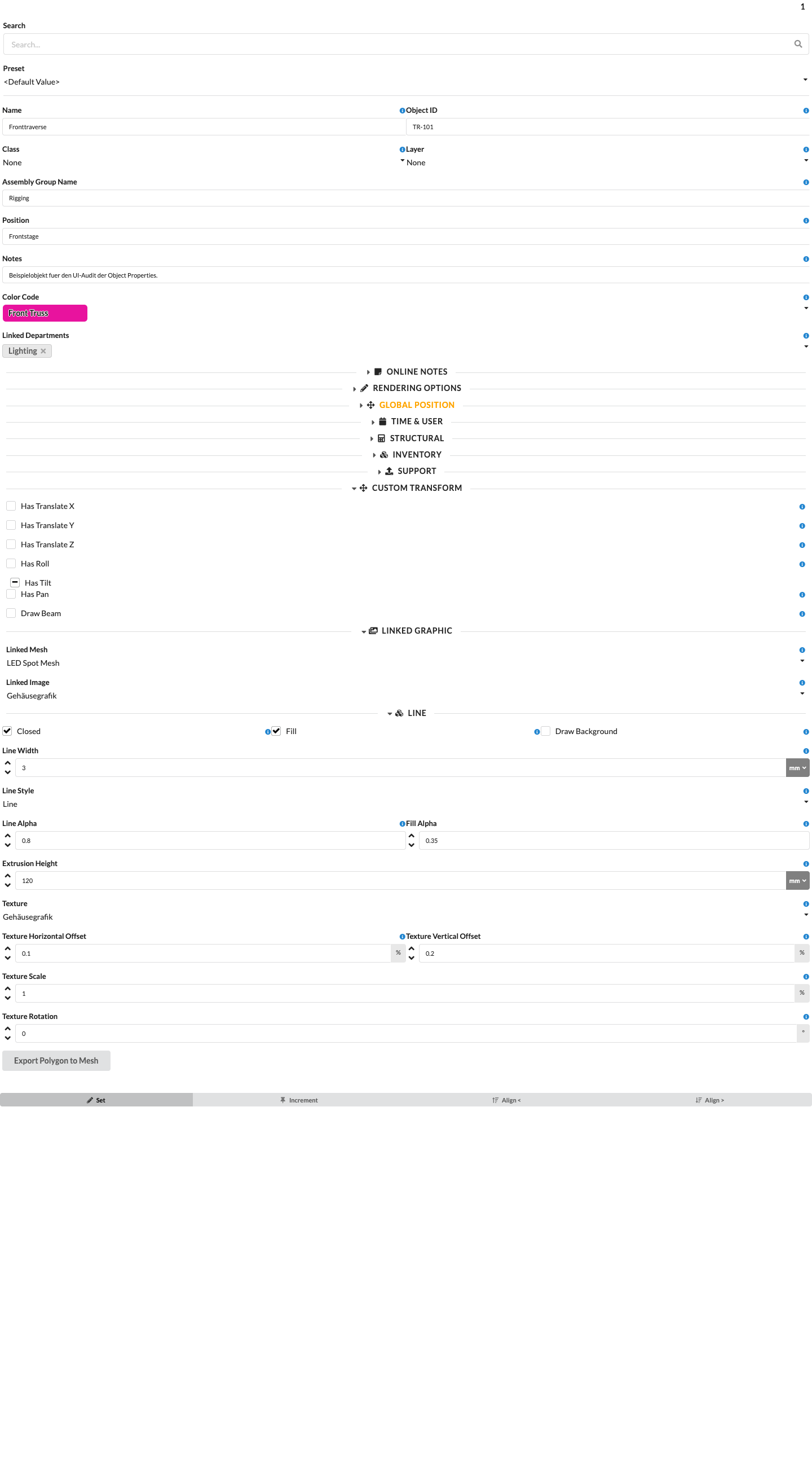
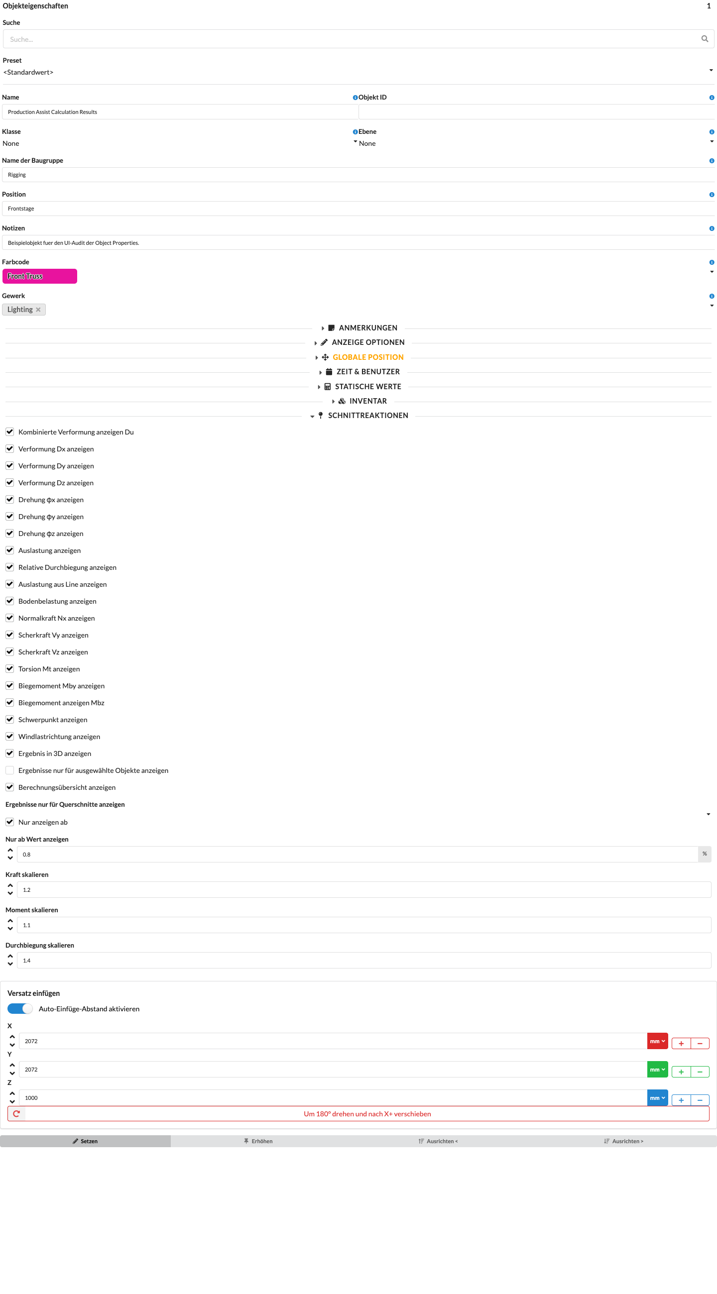
Select the Production Assist Calculation Results object in the Scene Tree and open Object Properties → Section Reactions to configure the displayed calculation results. Here you will find the same display options as in the Section Reactions tab in Navigation: result types, display scales, cross-section and object selection, and the minimum value filter. These settings change the display, not the calculation itself. Select the load combination used for the section reactions separately using the green dot in Navigation → Load Combinations. For detailed instructions, see Section Reactions; Load Combinations and Result Values explains how combinations map to results.
| Panel/Field | Detailed Description |
|---|---|
| Show Combined Deformation Du | Shows the resultant deformation of the cross-section. |
| Show Deformation Dx, Dy, Dz | Turns displacement components along the local X, Y, and Z axes on or off. |
| Show Rotation φx, φy, φz | Turns rotation components around the local axes on or off. |
| Show Utilization | Shows the calculated utilization. |
| Show Relative Deflection | Shows deflection relative to the span. |
| Show Utilization from Line | Shows the utilization from the line load display. |
| Show Ground Load | Shows or hides the displayed ground load. |
| Show Normal Force Nx | Shows or hides the normal force along the structure. |
| Show Shear Force Vy, Vz | Shows or hides the two shear force components. |
| Show Torsion Mt | Shows or hides the torsional moment. |
| Show Bending Moment Mby, Mbz | Shows or hides the bending moments around the local axes. |
| Show Center of Gravity | Shows or hides a black-and-white quartered circle with a magenta outline at the exact calculated center of gravity in the 3D renderer. For automatically braced XX rotation of a suspended truss arrangement, the roll inclination derived from the center-of-gravity position, an angle arc, and the value in degrees are also shown. This is not an FEM deformation rotation; see Load Centers of Gravity for prerequisites and special cases. |
| Show Wind Load Direction | Shows the direction of the wind loads taken into account. |
| Show Results in 3D | Controls how section reactions are displayed in the 3D model. |
| Show Results Only for Selected Objects | Limits the result display to currently selected objects. |
| Show Calculation Summary | Shows or hides the associated calculation summary. |
| Show Only for Cross-Sections | Limits the display to the selected cross-section. |
| Show Only From | Enables the minimum value filter for the result display. |
| Show Only Above Value | Sets the threshold for the minimum value filter. |
| Scale Force | Changes the display scale of forces. |
| Scale Moment | Changes the display scale of moments. |
| Scale Deflection | Changes the display scale of deformations. |
These sliders and checkboxes change only which results are displayed and at what scale. They do not affect the structural calculation or its results. The cross-section and minimum value filters can be used independently of each other.